0168
$$$B_{0}$$$-component determination of the gradient system transfer function using standard MR scanner hardware1Department of Diagnostic and Interventional Radiology, University Hospital Würzburg, Würzburg, Germany, 2X-Ray and Molecular Imaging Laboratory, Ostbayerische Technische Hochschule Amberg-Weiden, Weiden, Germany, 3Siemens Healthcare GmbH, Erlangen, Germany
Synopsis
As a linear and time-invariant (LTI) system, the dynamic gradient system can be described by the system transfer function. While special measurement equipment like field cameras can be used to precisely determine even higher orders of the transfer function, phantom-based approaches were introduced for alternative determination without additional hardware needed. This study reports on phantom-based measurements of B0-components, which resulted in transfer functions with sufficiently high resolution for the characterization of mechanical resonances.
Purpose
Dynamic gradient characteristics can be precisely measured using a field camera, which determines the transfer function of the gradient system1,2. Vannesjo et al.1 also utilized a field camera to determine B0-component characteristics of the gradient system response function (GIRF). With the phantom-based technique3,4 an alternative method was introduced which is capable of acquiring gradient system transfer characteristics with no need for additional measurement hardware. In the past, this phantom-based technique was used for, e.g., trajectory correction by determining linear terms of the GIRFs in its three spatial dimensions4-6. In this study, the phantom-based method was used to determine and evaluate B0-components of the gradient system transfer function (GSTF).Methods
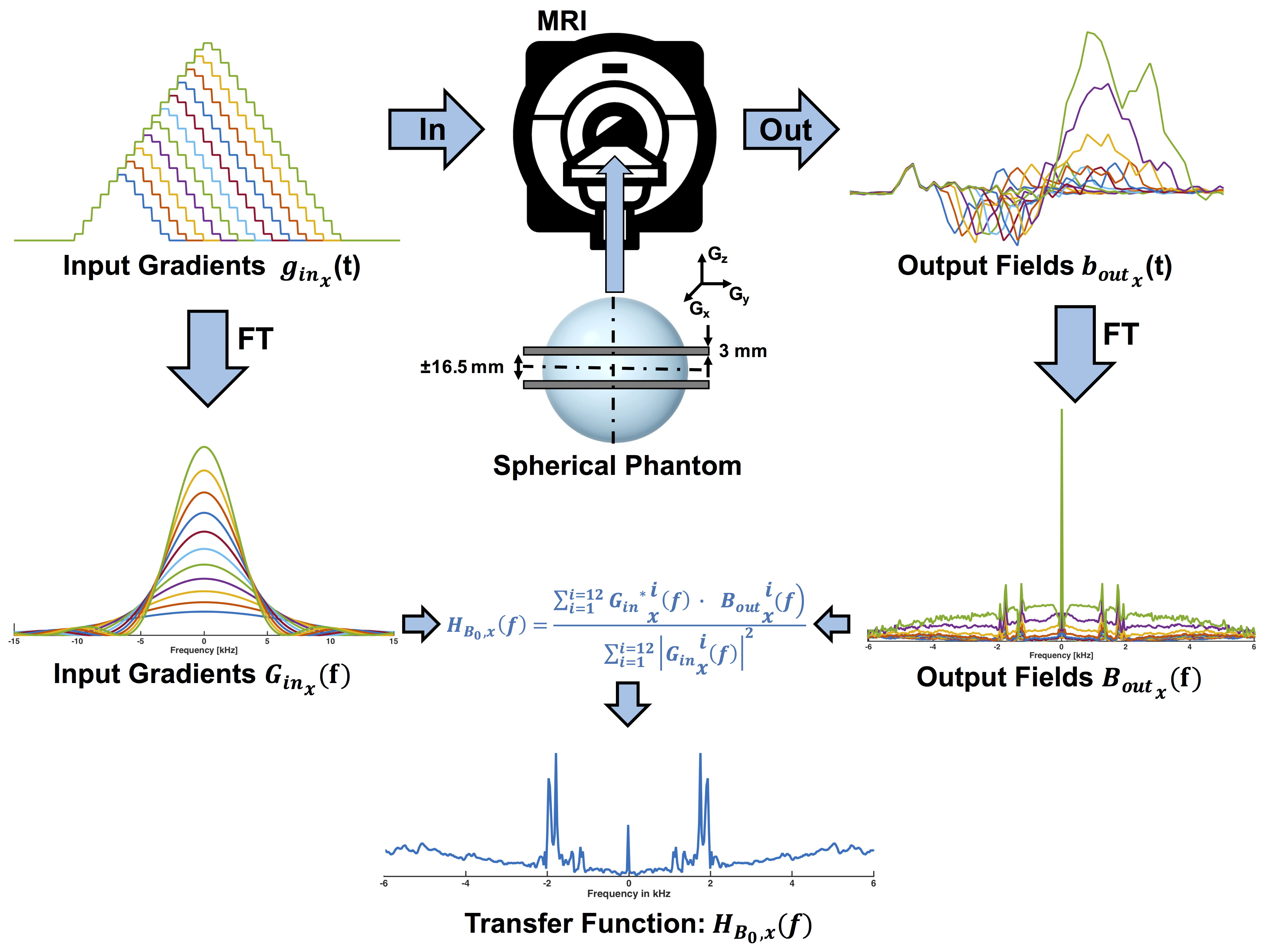
Experiments were performed with a spherical phantom placed inside a 3T Siemens MAGNETOM Prismafit scanner (Siemens Healthcare, Erlangen, Germany). In a prototype sequence, 12 different input gradients $$$g_{in}(t)$$$ (duration 100 – 320 µs, slew rate = 180 T/m/s) with broad spectral support were played out. The responding phases $$$\Phi_{1}(t)$$$ and $$$\Phi_{2}(t)$$$ were measured in two parallel slices at position ±16.5 mm, vertical to the input gradient direction. For each slice, a reference phase $$$\Phi_{.,ref}(t)$$$ was additionally acquired with no gradient waveforms played out by the system. The gradient system response $$$b_{out}(t)$$$ for linear GSTF components are determined as the difference in phase evolution. In contrast to that, the gradient system response $$$b_{out}(t)$$$ for the determination of B0-components can then be calculated from the sum of the phase evolution:
$$b_{out}(t)=\frac{1}{2} \cdot \frac{1}{\gamma} \cdot \frac{d}{dt}[(\Phi_{1}(t)-\Phi_{1,ref}(t))+(\Phi_{2}(t)-\Phi_{2,ref}(t))].$$
Finally, the B0-components of the transfer functions can then be calculated as:
$$H_{B_{0},k}(f)=\frac{\sum_{i=1}^N {G_{in}^{*}}_{k}^{i}(f) \cdot {B_{out}}_{k}^{i}(f)}{\sum_{i=1}^N {{G_{in}}_{k}^{i}(f)}^2},$$
where $$$k$$$ represents the direction in which the input gradient is played out. The index represents a particular triangular waveform, and $$$N$$$ the total number of input gradients. $$$G_{in}(f)$$$ and $$$B_{out}(f)$$$ are the Fourier transforms of $$$g_{in}(t)$$$ and $$$b_{out}(t)$$$.
Relevant measurement parameters were set to: TR = 5.0 s, slice thickness = 3 mm, slice positions = ±16.5 mm, flip-angle = 90°, bandwidth = 119 kHz, 40 averages. The length of the acquisition window was ~33 ms such that the GSTF featured a frequency resolution of 30 Hz. The complete acquisition of one B0-component takes about 70 min. Fig. 1 visualizes the B0-component measurement and calculation process schematically.
Results
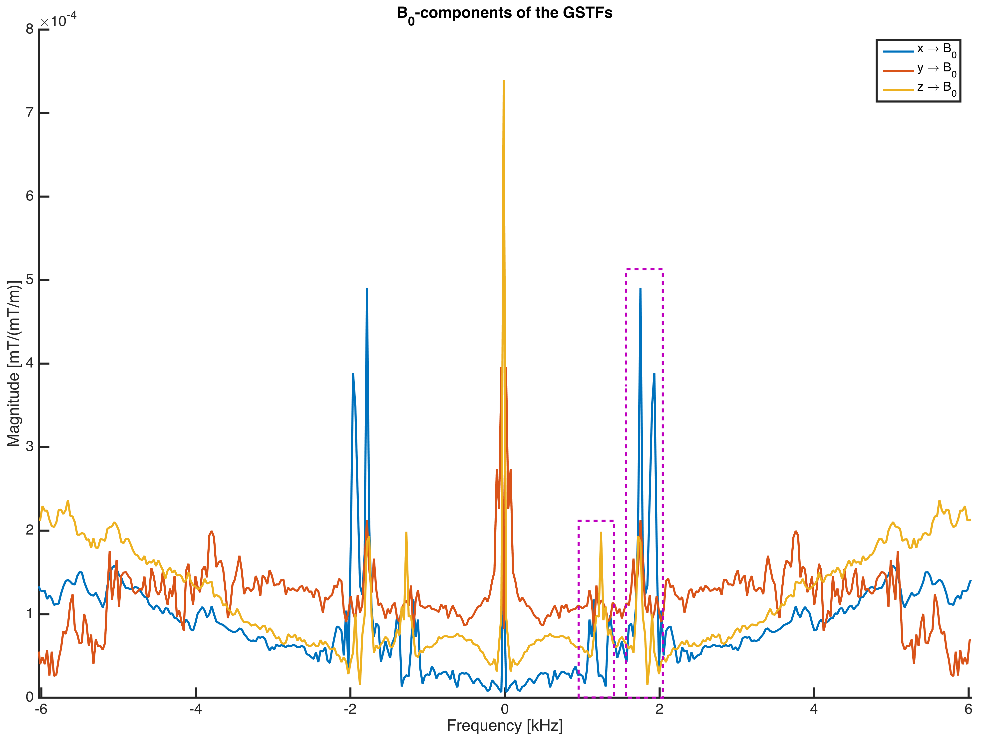
The measured B0-component transfer functions of all three spatial dimensions are shown in Fig. 2 for the frequency range between -6 kHz and 6 kHz. The magnitude is specified with the unit [mT/(mT/m)]. Several peaks can be seen, which are probably caused by mechanical resonances. Resonance areas are in ranges of 1.0-1.4 kHz and 1.7-2.2 kHz and marked with dotted purple rectangles. The x-axis component shows the strongest response on the input gradients in the range of 1.7-2.2 kHz, with magnitudes about twice the size of the z-axis component. The y-axis component indicates the smallest resonance response.Discussion & Conclusion
The B0-component characteristics, which are determined in this study, are comparable to those acquired with a field camera in a different 3T MR system1. The proposed procedure therefore represents a comparably simple and robust alternative technique, which is independent from additional measurement hardware. Together with the linear-term GSTFs, the B0-component GSTFs can e.g. be applied for the correction of non-Cartesian trajectories or for the correction of phase shifts in balanced Steady-State-Free-Precession (bSSFP) imaging7.Acknowledgements
No acknowledgement found.References
1. Vannesjo SJ, Haeberlin M, Kasper L, et al. Gradient system characterization by impulse response measurements with a dynamic field camera. Magn Reson Med 2013;69:583–593.
2. Vannesjo SJ, Graedel NN, Kasper L, et al. Image Reconstruction Using a Gradient Impulse Response Model for Trajectory Prediction. Magn Reson Med 2016 Jul;76:45-58.
3. Liu H, Matson GB Accurate Measurement of Magnetic Resonance Imaging Gradient Characteristics. Materials (Basel). 2014;7(1):1–15.
4. Campbell-Washburn AE, Xue H, Ledermann RJ, et al. Real-time distortion correction of spiral and echo planar images using the gradient system impulse response function. Magn Reson Med 2016;75:2278–2285.
5. Stich M, Wech T, Slawig A, et al. Implementation of a Gradient Pre-emphasis Based on the Gradient Impulse Response Function. Proceedings ISMRM 2017;3909.
6. Stich M, Wech T, Ringler R, et al. Implementation of a Gradient Waveform Pre-emphasis Based on the Gradient Impulse Response Function for a Spiral Sequence. Magn Reson Mater Phy. 2017;30:71.
7. Fischer RF, Barmet C, Rudin M, et al. Monitoring and compensating phase imperfections in cine balanced steady-state free precession. Magn Reson Med. 2013;70:1567-1579.
Figures