0166
Constrained MRSI Reconstruction Using Water Side Information with a Kernel-Based Method1Department of Electrical and Computer Engineering, University of Illinois at Urbana-Champaign, Urbana, IL, United States, 2Beckman Institute for Advanced Science and Technology, University of Illinois at Urbana-Champaign, Urbana, IL, United States, 3Paul C. Lauterbur Research Center for Biomedical Imaging, Institutes of Advanced Technology, Shenzhen, China
Synopsis
Reconstruction for MR spectroscopic imaging (MRSI) is a challenging problem where incorporation of spatiospectral prior information is often necessary. While spectral constraints have been effectively utilized in the form of temporal basis functions, spatial constraints are often imposed using spatial regularization. In this work, we present a new kernel-based method to incorporate a priori spatial information, which was motivated by the success of kernel-based methods in machine learning. It provides a new mechanism for constrained image reconstruction, effectively incorporating a priori spatial information. The proposed method has been evaluated using both simulation and in vivo data, producing very impressive results. This new reconstruction scheme can be used to process any MRSI data, especially those from high-resolution MRSI experiments.
Introduction
A major practical problem with magnetic resonance spectroscopic imaging (MRSI) is low signal-to-noise ratio (SNR). To improve image reconstruction, it is often necessary to incorporate a priori spectral and/or spatial constraints. While spectral constraints have been effectively utilized in the form of temporal basis functions derived from training data, spatial constraints are often imposed using spatial regularization1-3. In this work, we present a new kernel-based method to incorporate a priori spatial information. This method was motivated by the success of kernel-based methods in machine learning4. It provides a new mechanism for constrained image reconstruction, effectively incorporating a priori spatial information. The performance of the proposed method has been evaluated using both simulated and in vivo MRSI data, producing very encouraging results.Method
Kernel-based signal model
Exploiting the partial separability (PS) property of MRSI signals, the desired spatiotemporal function can be expressed as5
$$\hspace{8em}s(\boldsymbol{x}_n,t_m)=\sum_{l=1}^{L}c_{l}(\boldsymbol{x}_n)\psi_{l}(t_m),\hspace{0.3em}n=1,2,...,N\hspace{0.3em}\mathrm{and}\hspace{0.3em}m=1,2,...,M\hspace{7.5em}(1)$$
where $$$L$$$ is usually a small number in practice, $$$\{\psi_l(t_m)\}_{l=1}^L$$$ are temporal basis functions and $$$\{c_{l}(\boldsymbol{x}_n)\}_{l=1}^{L}$$$ the corresponding spatial coefficients.
In the previous works2-3, the $$$c_l(\boldsymbol{x}_n)$$$ is represented using the conventional Fourier model; in this work, we use a kernel-based model to represent $$$c_l(\boldsymbol{x}_n)$$$. More specifically, we assume that $$$c_{l}(\boldsymbol{x}_n)$$$ at each location $$$\boldsymbol{x}_n$$$ can be viewed as a function of a set of low-dimensional features $$$\hspace{0.2em}\boldsymbol{f}_n\in\mathbb{R}^p$$$:
$$\hspace{16.6em}c_{l}(\boldsymbol{x}_n)=\Omega_l(\boldsymbol{f}_n).\hspace{16.6em}(2)$$
The features $$$\{\boldsymbol{f}_n\}_{n=1}^N$$$ can be extracted or "learned" from water images (such as those obtained from a reference scan or the companion water images in MRSI experiments without water suppression). However, $$$\Omega_l(\cdot)$$$ is often highly complex in practice and cannot be accurately described as a linear operator in the original feature space4,6-7. Inspired by the "kernel trick" in machine learning, we express $$$\Omega_l(\cdot)$$$ in a transformed space spanned by $$$\{\phi(\boldsymbol{f}_n):\boldsymbol{f}_n\in{\mathbb{R}^p}\}$$$ as:
$$\hspace{16.2em}\Omega_l(\boldsymbol{f}_n)=\omega_l^T\phi(\boldsymbol{f}_n),\hspace{16.2em}(3)$$
where $$$\phi(\cdot)$$$ is some mapping function. The well-known representer theorem ensures that the optimal $$$\omega_l$$$ takes the following form8:
$$\hspace{16.25em}\omega_l=\sum_{i=1}^N\alpha_{l,i}\phi(\boldsymbol{f}_i).\hspace{16.25em}(4)$$
Hence we obtain the kernel representation for $$$c_l(\boldsymbol{x}_n)$$$ as
$$\hspace{11.6em}c_l(\boldsymbol{x}_n)=\sum_{i=1}^N\alpha_{l,i}\phi^T(\boldsymbol{f}_i)\phi(\boldsymbol{f_n})=\sum_{i=1}^N\alpha_{l,i}k(i,n),\hspace{11.6em}(5)$$
where $$$k(i,n)=\phi^T(\boldsymbol{f}_i)\phi(\boldsymbol{f_n})$$$ is a kernel function. Substituting Eq. (5) into Eq. (1) leads to the kernel-based representation for the MRSI signals:
$$\hspace{12.8em}s(\boldsymbol{x}_n,t_m)=\sum_{l=1}^{L}\{\sum_{i=1}^N\alpha_{l,i}k(i,n)\}\psi_{l}(t_m).\hspace{12.8em}(6)$$
The equivalent matrix-vector form of Eq. (6) is
$$\hspace{17.5em}\boldsymbol{s}=KA\Psi,\hspace{17.5em}(7)$$
where $$$A\in\mathbb{C}^{N×L}$$$ is formed by $$$\{\alpha_{l,i}\}$$$ appropriately. Note that each column of $$$K$$$ can also be viewed as a spatial basis function.
Kernel-based Image Reconstruction
As in the existing works, the temporal basis functions in Eq. (6) are determined from training data2-3. To determine the kernel matrix, we choose the radial Gaussian kernel function:
$$k(\boldsymbol{f}_i,\boldsymbol{f}_j)=\exp(-\frac{||\boldsymbol{f}_i-\boldsymbol{f}_j||_2^2}{2\sigma^2}),$$
which corresponds to an infinite-dimensional mapping function. The image feature vectors $$$\{\boldsymbol{f}_i\}$$$ contain image intensities and edge information.
After $$$K$$$ is determined, kernel-based reconstruction for MRSI is performed using a penalized maximum likelihood (ML) formulation. Specifically, we solve the following regularized least-squares problem:
$$\hspace{10.25em}\{A^*\}=\min_{\{A\}}||d-ΠF_B{KA\Psi}||_2^2+{\lambda}R(A),\hspace{10.25em}(8)$$
where $$$d$$$ is the measured MRSI data, $$$Π$$$ the k-space sampling operator, $$$F_B$$$ the Fourier encoding operator including B0 inhomogeneity, $$$R(A)$$$ a regularization term and $$$\lambda$$$ a tunable parameter. Many choices can be used for $$$R(A)$$$, and in this work we choose $$$R(A)=||KA\Psi-\hat{S}||$$$ where $$$\hat{S}$$$ is the initial reconstruction obtained by the use of edge-preserving regularization. But note that $$$R(A)$$$ mainly serves to improve the conditioning rather than imposing spatial smoothing, as in the standard regularization techniques. The final reconstruction of the desired spatiotemporal function can be obtained by substituting $$$A^*$$$ into Eq. (7).
Results
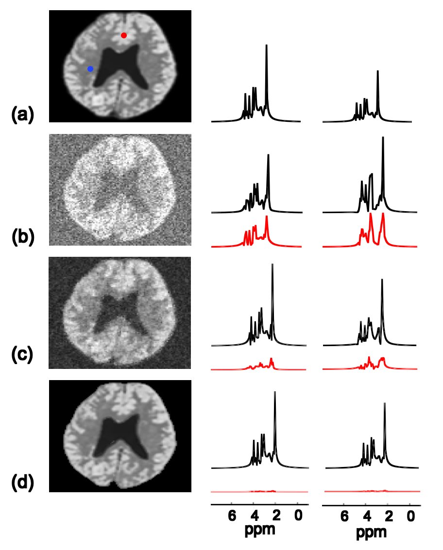
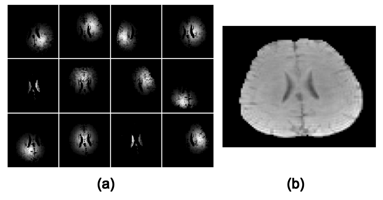
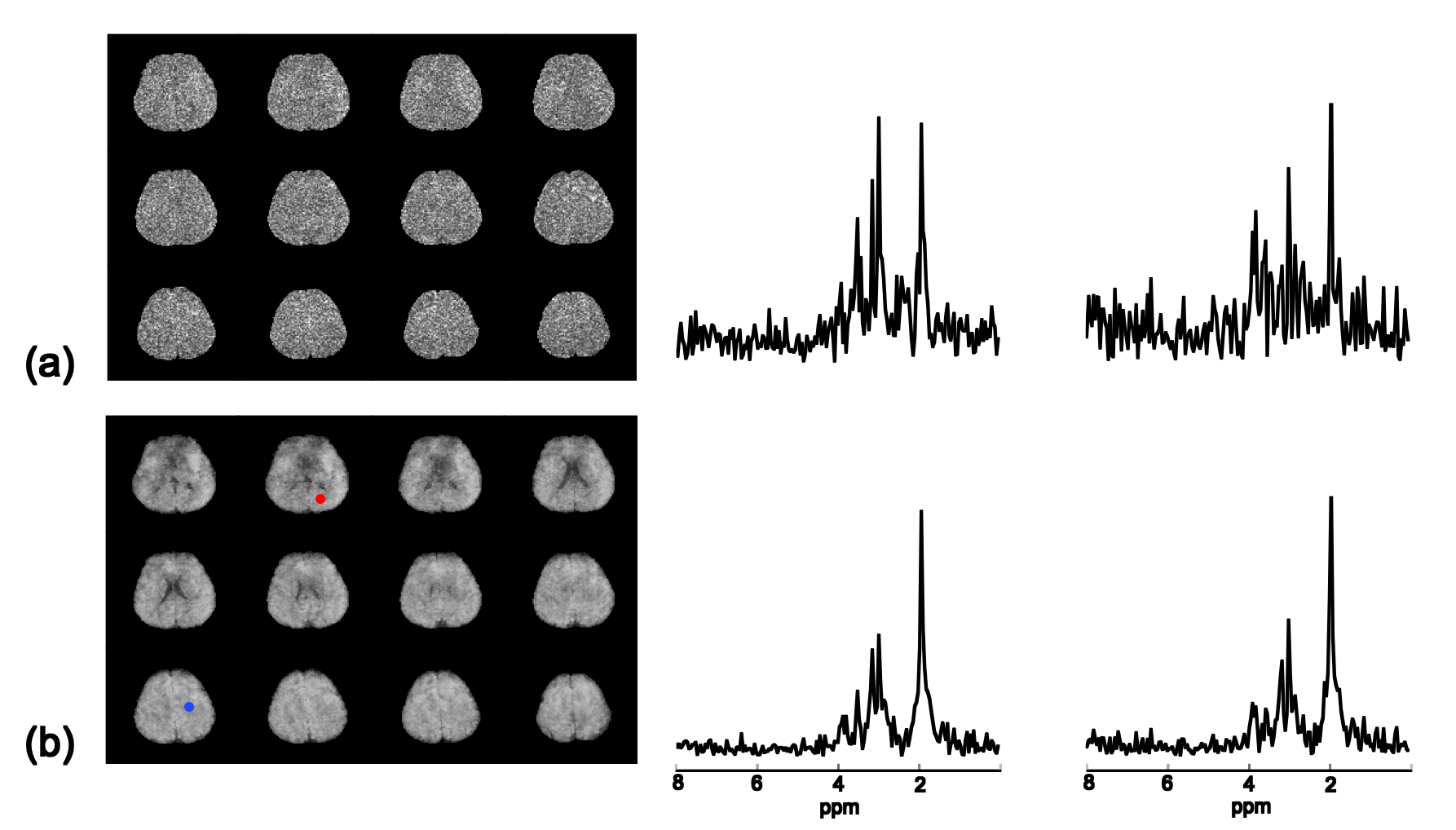
The proposed method has been validated using both simulated and in vivo data. The simulation data were generated from a computational phantom containing spatial distributions of common metabolites plus Gaussian noise. Figure 1 illustrates the comparison between the proposed method and other existing reconstruction methods, including subspace projection (i.e. directly projecting the spatiospectral distributions onto the subspace spanned by $$$\{\psi_l(t_m)\}_{l=1}^L$$$) and a spatially regularized method. The results demonstrate that the proposed method has significantly higher reconstruction accuracy. In vivo data were acquired from a healthy human subject using the SPICE technique2-3 with the following imaging parameters: TR/TE=300/4 ms, 230×230×72 mm3 FOV and 96×110×24 matrix size. Figure 2 shows a sample of spatial basis functions obtained by reshaping different columns of $$$K$$$, which demonstrates how the water side information is incorporated into the signal model. Figure 3 shows that the reconstruction by subspace projection has much larger spatiospectral variations, which have been significantly reduced by the proposed method.Conclusions
This paper presents a new kernel-based method for constrained MRSI reconstruction that incorporates water side information into the signal model. The proposed model represents the spatial coefficients of the PS spatiospectral model as kernel functions of anatomical image features. The method has been evaluated using both simulation and in vivo data, producing impressive results. It can be used to process any MRSI data, especially those from high-resolution experiments.Acknowledgements
This work was supported in part by the following grants: NIH-R21-EB021013-01 and NIH-P41-EB002034.References
1. Kasten, J., Lazeyras, F., & Van De Ville, D. (2013). Data-driven MRSI spectral localization via low-rank component analysis. IEEE transactions on medical imaging, 32(10), 1853-1863.
2. Lam, F., & Liang, Z. P. (2014). A subspace approach to high‐resolution spectroscopic imaging. Magnetic resonance in medicine, 71(4), 1349-1357.
3. Lam, F., Ma, C., Clifford, B., Johnson, C. L., & Liang, Z. P. (2016). High‐resolution 1H‐MRSI of the brain using SPICE: Data acquisition and image reconstruction. Magnetic resonance in medicine, 76(4), 1059-1070.
4. Chen, P. H., Lin, C. J., & Schölkopf, B. (2005). A tutorial on ν‐support vector machines. Applied Stochastic Models in Business and Industry, 21(2), 111-136.
5. Liang, Z. P. (2007). Spatiotemporal imaging with partially separable functions. In IEEE International Symposium on Biomedical Imaging, Arlington, VA, USA, 2007, 988-991.
6. Wang, G., & Qi, J. (2015). PET image reconstruction using kernel method. IEEE transactions on medical imaging, 34(1), 61-71.
7. Novosad, P., & Reader, A. J. (2016). MR-guided dynamic PET reconstruction with the kernel method and spectral temporal basis functions. Physics in medicine and biology, 61(12), 4624.
8. Schölkopf, B., Herbrich, R., & Smola, A. (2001). A generalized representer theorem. In Computational learning theory (pp. 416-426). Springer Berlin/Heidelberg.
Figures