0162
Metabolite Quantification of 1H-MRSI spectra in Multiple Sclerosis: A Machine Learning Approach1Department of Computer Science, Technical University of Munich, Munich, Germany, 2Institute for Digital Communications, University of Edinburgh, Edinburgh, Scotland, 3Centre for Clinical Brain Sciences, University of Edinburgh, Edinburgh, Scotland, 4Queen Square Multiple Sclerosis Centre, Department of Neuroinflammation, University College London, London, United Kingdom
Synopsis
As an alternative to model-based spectral fitting tools, we introduce a machine-learning framework for estimating metabolite concentrations in MR spectra acquired from a homogeneous cohort of 42 patients with Secondary Progressive Multiple Sclerosis. Our framework based on random-forest regression performs a 42-fold cross validation on this dataset which involves (1) learning the spectral features from this cohort; (2) estimating concentrations and calculating relative error over the LCModel estimates. Compared to the LCModel, our method, after training, gives a low estimation error and a 60-fold improvement in estimation speed per patient.
Purpose
Multiple Sclerosis (MS) is an inflammatory neurological diseases affecting around 2.5 million people globally (www.mstrust.org.uk). Quantification of metabolites can yield important diagnostic information about disease progression for which model-based fitting tools such as the LCModel1 are widely used. Despite being the gold-standard, they require prior knowledge-tuning and can also be time-consuming. Prior work on healthy human brains has shown Random-Forest regression to perform the same quantification but at a faster speed2. The purpose of this work is to apply this method to a clinical setup involving MS-patients and address the limitations of parameter-tuning and speed of conventional fitting tools by validating on an extensive $$$^1$$$H MRSI-MS dataset.Methods
Random Forests3 have been shown to be effective in a wide range of classification4,5 and regression problems2, including classification of MS-spectra6. These involve multiple forests comprising of a set of binary trees. For training, splits are created in each tree based on random subsets of the feature variables and piecewise linear regression is performed over the input data2. The process involves seeking best prediction at every node and using thresholding to further propagate data points till they reach the end of the tree. Subsequently the weighted average of the prediction from each tree is taken to give a single output estimate.In MRSI, the time-domain complex signal of a nucleus is given by: $$S(t)=\int \mathrm{p}(\omega)\mathrm{exp}(-i\Phi)\mathrm{exp}(-t/T^{*}_{2})dw.$$, and the corresponding frequency-domain spectrum is given by $$$S(\omega)$$$. As shown in Fig.1, we aim to perform the inverse signal-modeling where we have a training dataset, $$$D=(S_{i} (\omega), Y_{i}), i\in [1, N]$$$,where $$$N $$$ is the total number of MS training spectra from 41 patients. $$$S_{i}(\omega)$$$ represents the training spectral data while $$$Y_{i}$$$ represents the corresponding multi-parameter training labels. For our model, we consider the absolute concentrations of NAA, Cho, Cr, myo-inositol(mI) and glutamate+glutamine (Glx). Therefore, for a given spectrum $$$S_{i}(\omega)$$$, $$$Y_{i} = [NAA_{i}, Cho_{i}, Cr_{i}, mI_{i}, Glx_{i}]$$$.
We run a K-Fold cross validation with 42 folds, number of trees = $$$100$$$ and mTry = $$$128$$$ to generate training sets using spectra from 41 patients and test on the spectra, $$$S_{j}(\omega)$$$, from the remaining patient to obtain concentration estimates $$$\hat{Y}_{j}$$$. The corresponding LCModel fitted concentration labels $$$Y_{j}$$$ serve as the ground-truth, $$$j\in [1, M]$$$ where $$$M$$$ is the total number of test spectra.
Error Calculation. For our experiments, we assess the absolute relative change in parameter estimates over the ground-truth values. Given the estimate $$$\hat{Y}_{j}$$$ and the testing label $$$Y_{j}$$$, the estimate error for the parameter $$$Y_{j}$$$ can be calculated as,$$\hat{E}_{j} = ||\hat{Y}_{j} - Y_{j}||./||Y_{j}||$$
Subjects. 42 patients (age 55±8) with Secondary Progressive Multiple Sclerosis (SPMS) (EDSS score 6±0.7) were recruited as part of the study. The patients underwent MRI examination at 3T, including T1w, T2w and FLAIR scans and proton semi-LASER MRSI with $$$TR/TE = 2000/43 ms$$$ and $$$481$$$ data points over spectral region-of-interest. An example has been shown in Fig.2. Prior work provides additional acquisition details7. The data was fitted using LCModel and the voxels which did not pass the Cramer-Rao Lower Bound (CRLB) and visual quality tests were discarded (e.g. distorted baselines). There are no 'pure' lesion or non-lesion voxels and therefore all spectra are of mixed content. Total spectra per fold included approximately $$$4200$$$ training and $$$100$$$ test-spectra/patient respectively.
Results
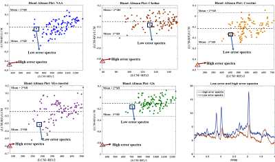
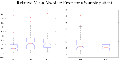
We aim to get an error $$$\hat{E}_{j}$$$ of $$$<15{\%}$$$ for each of the metabolites per patient. The mean absolute relative error plots for all patients are shown in Fig.3. Using the Bland-Altman method8, we observe a strong correlation between the LCModel and RF estimates for a sample patient (Fig.4). $$$\hat{E}_{j}$$$ for the same sample patient are within the acceptable range (especially for the major metabolites such as NAA, Choline and Creatine)(Fig.5).
Speed: Training time per fold is 3 minutes. While the LCModel takes 10 minutes per patient for the metabolite quantification, our proposed framework, after training, takes only $$$10 sec$$$ leading to a $$$60x$$$ improvement in speed
Discussion and Conclusion
An outlier high-error spectrum for a test-patient has been highlighted in Fig.4 which corresponds to the outlier whisker in Fig.5. The peaks in this spectrum are not well-defined and only few such spectra are present in the training set. The machine learning algorithm is therefore insufficiently trained on such spectra resulting in a high error. Future work would involve using a more robust approach such as deep-learning based methods to improve the accuracy of parameter estimation. Once a framework has been established, further work can be done on having a MS-specific simulated spectra model with wider variations in the spectral peak for parameter estimation to predict disease progression and the corresponding metabolite maps.Acknowledgements
Spectral data were provided by the MS-SMART consortium (www.ms-smart.org). The research leading to these results has received funding from the European Union's H2020 Framework Programme (H2020-MSCA-ITN-2014) under grant agreement n° 642685 MacSeNet.References
1. Provencher SW. Estimation of metabolite concentrations from localized in-vivo proton NMR spectra. Magnetic Resonance in Medicine (6), 672-679 (1993).
2. Das, D., Coello, E., Schulte, R.F., Menze, B.H.: Quanti fication of Metabolites in Magnetic Resonance Spectroscopic Imaging Using Machine Learning, pp. 462-470. Springer International Publishing, Cham (2017).
3. Breiman, L.: Random forests. Machine Learning 45(1), 5{32 (2001).
4. Pedrosa de Barros, N., McKinley, R., Wiest, R., Slotboom, J.: Improving labeling efficiency in automatic quality control of MRSI data. Magnetic Resonance in Medicine.(2017)
5. Menze, B.H., Kelm, B.M., Weber, M.A., Bachert, P., Hamprecht, F.A.: Mimicking the human expert: Pattern recognition for an automated assessment of data quality in MR spectroscopic images. Magnetic Resonance in Medicine 59(6), 1457-1466 (2008).
6. Ion-Mrgineanu, A., Kocevar, G., Stamile, C., Sima, D.M., Durand-Dubief, F.,Van Huffel, S., Sappey-Marinier, D.: Machine learning approach for classifying multiple sclerosis courses by combining clinical data with lesion loads and magnetic resonance metabolic features. Frontiers in Neuroscience 11, 398 (2017).
7. Marshall I et al., Proc ISMRM 2017; 4639.
8. Bland, J.M., Altman, D.: Statistical methods for assessing agreement between two methods of clinical measurement. The Lancet 327(8476), 307-310 (1986).
Figures
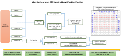
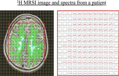
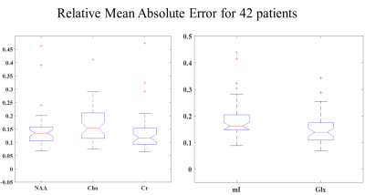
Fig.3: Absolute Relative Error box-plots for the entire 42-patient spectra dataset. The mean relative errors are: (Left) NAA (13.4%), Choline (13.8%), Creatine (10.8%); (Right) mI (14.7%), Glx (10.8%). 5 of the patient data included outlier spectra similar to the one shown in Fig. 4 which led to an overall increase in the mean relative errors for each of the metabolites.
