0155
A transfer function model for local signal propagation in spatiotemporal MR data1Weill Cornell Medicine, New York, NY, United States, 2Leibniz Institute for Neurobiology, Magdeburg, Germany
Synopsis
In order to understand the sources of dynamic EPI signals under complex stimuli or in the resting state, local signal transfer functions were computed from natural stimulation data sets, and the coherence vector was mapped and color coded analogously to conventional methods for structural connectivity maps. As expected, signal propagation is frequency dependent, whereas high frequencies are caused by cardiovascular pulsations, but low frequencies are less well understood. We conclude that the observed frequency dependence of this local signal transfer model might aid the understanding of the foundation of functional connectivity analysis and the meaning of observed complex patterns such as the resting states.
Introduction
Functional MR imaging provides spatiotemporal (3D & time) data sets whose full complexity under various tasks or even during ‘rest’ we are just starting to appreciate. In addition, EPI-based fMRI experiments increasingly move from tightly controlled designs to experiments that probe the brain under natural, complex stimuli or behavior, such as virtual reality or watching movies. In order to understand brain activity in these experiments, it is even more important to be able to disentangle the various contributions to the spatiotemporal EPI signals1. Towards this end, here we performed an analysis of local signal propagation2,3 between neighboring MRI voxels by means of transfer functions and coherences. This method might aid the detection of local EPI signal properties of relevance for global connectivity studies4 by mapping frequency-dependent EPI signal sources, for example vascular vs. BOLD sources.
Methods
Theory: The linear relationship, including arbitrary lag times, between an output signal y(t) and an input signal x(t) can be written in frequency space under steady-state conditions by the transfer or frequency response function H(ω), which relates the Fourier transforms X(ω) and Y(ω) to each other, i.e.,
Y(ω) = H(ω)X(ω) .
Here, the signals consists of time series of EPI data, independent of their origin (vascular, BOLD, flow, etc.) With the cross- and auto-power spectra PXY(ω) = X*(ω)Y(ω), PXX(ω) = |X(ω)|2, PYY(ω) = |Y(ω)|2, the coherence between the signals is
CXY(ω) = |PXY(ω)|2/(PXX(ω)PYY(ω)) = |H(ω)|2 PXX(ω)/PYY(ω).
The application to spatiotemporal data is shown schematically in Figure 1, which also includes further model assumptions.
Data: Four natural stimulation (audio version of a feature film) dynamic EPI scans from a publicly available data base5 were used, covering parts of frontal and occipital cortex and regions in between. The data was acquired on a 7 Tesla MRI scanner and sampled every 2 s for 15 min at 1.4 mm isotropic resolution.
Analysis: Local coherences of the EPI signal were obtained from high-pass filtered data (cutoff period 1 min to remove trends6,7), using standard spectral estimation methods as they are provided by Matlab’s cpsd function. For each voxel, three nearest neighbor coherences were taken into account (to avoid redundancy) and a coherence vector formed from these. The vector magnitude was represented as maximum intensity projections (MIPs), and the principal direction (largest of the three components) color coded analogously to methods used for structural connectivity maps8.
Results
Signal propagation is visible at the main cerebral arteries, in smaller arteries, next to or in gray cortical matter, in cerebrospinal fluid, and in some extracerebral areas, but mostly absent in white matter (Figures 2, 3). This signal propagation is frequency dependent: For high frequencies (corresponding periods below 12.5 s), mainly the main arteries are visible, for lower frequencies (periods between 12.5 and 60 s), smaller arteries and probably some gray matter areas are added while the main blood vessels appear diminished but not completely suppressed. The gray matter of the basal ganglia and thalamus does not show pronounced signal transfer in this model. There are also artifacts caused but not limited to eye and head motion. The model’s sensitivity becomes apparent when applied to data sets that underwent widely used standard fMRI pre-processing: Re-sampling data to higher resolution and distortion correction cause artifacts, shown in Figure 2D.
Discussion
The cardiac pulse affects mainly the highest frequencies of the EPI signal. This pulse sensitivity has been observed before in complementary local methods tailored to pulsatile signals in EPI data9-11. Low-frequency fluctuations visible in signal transfer12 seemingly affect smaller vessels and gray matter, but their origin (autoregulation/neuronal processes or their interaction13) and their exact source (arterioles/veins/capillary bed) remain open without further analysis or experiments. The possible value of color coding the direction of the coherence vector still needs to be evaluated. In order to avoid some of the present model assumptions (Figure 1), partial coherences14,15 could be used, and for more than three directions.
Conclusion
The observed frequency dependence of a local signal transfer model for spatiotemporal MR data might aid the understanding of the foundation of applications such as functional connectivity analysis and the meaning of observed complex patterns such as the resting states. The proposed model might be the starting point for a more refined analysis, with possible value towards the interpretation16-18 of the growing number of clinical and more complex MRI experiments or the application of network control theory to the human brain19. In addition, vectorizing3 local neuronal connectivity is a first step towards tracking of functional connections in gray matter analogous to tracking structural connections in white matter, and thus again a step towards a global mapping of brain dynamics.
Acknowledgements
We would like to thank M. Hanke and A. Brechmann for personal support.
References
1 Birn, R. M., Diamond, J. B., Smith, M. A. & Bandettini, P. A. Separating respiratory-variation-related fluctuations from neuronal-activity-related fluctuations in fMRI. NeuroImage 31, 1536-1548 (2006).
2 Voss, H. U., Helekar, S. A. & Schiff, N. D. Local spatial synchronization fMRI indicates functional specialization of putamen in motor imagery. Proc. Human Brain Mapping (2014).
3 Voss, H. U. & Schiff, N. D. Searching for conservation laws in brain dynamics-BOLD flux and source imaging. Entropy 16, 3689-3709 (2014).
4 Sporns, O. Networks of the Brain. (MIT Press, 2011).
5 Hanke, M. et al. A high-resolution 7-Tesla fMRI dataset from complex natural stimulation with an audio movie. Scientific Data 1 140003, doi:10.1038/sdata.2014.3 (2014).
6 Biswal, B., Yetkin, F. Z., Haughton, V. M. & Hyde, J. S. Functional connectivity in the motor cortex of resting human brain using echo-planar MRI. Magn. Reson. Med. 34, 537-541 (1995).
7 Greicius, M. D. & Menon, V. Default-mode activity during a passive sensory task: Uncoupled from deactivation but impacting activation. J. Cogn. Neurosci. 16, 1484-1492 (2004).
8 Pajevic, S. & Pierpaoli, C. Color schemes to represent the orientation of anisotropic tissues from diffusion tensor data: Application to white matter fiber tract mapping in the human brain. Magn. Reson. Med. 42, 526-540 (1999).
9 Tong, Y. J., Hocke, L. M. & Frederick, B. D. Short repetition time multiband echo-planar imaging with simultaneous pulse recording allows dynamic imaging of the cardiac pulsation signal. Magn. Reson. Med. 72, 1268-1276, doi:10.1002/Mrm.25041 (2014).
10 Dagli, M. S., Ingeholm, J. E. & Haxby, J. V. Localization of cardiac-induced signal change in fMRI. NeuroImage 9, 407-415, doi:10.1006/nimg.1998.0424 (1999).
11 Voss, H. U., Dyke, J. P., Tabelow, K., Schiff, N. D. & Ballon, D. J. Magnetic resonance advection imaging of cerebrovascular pulse dynamics. J. Cereb. Blood Flow Metab. 37, 1223-1235, doi:10.1177/0271678x16651449 (2017).
12 Drew, P. J., Duyn, J. H., Golanov, E. & Kleinfeld, D. Finding coherence in spontaneous oscillations. Nat. Neurosci. 11, 991-993, doi:10.1038/nn0908-991 (2008).
13 Pfurtscheller, G. et al. Distinction between neural and vascular BOLD Oscillations and intertwined heart rate oscillations at 0.1 Hz in the resting state and during movement. PLoS ONE 12, doi:10.1371/journal.pone.0168097 (2017).
14 Zhou, D. L., Thompson, W. K. & Siegle, G. MATLAB toolbox for functional connectivity. NeuroImage 47, 1590-1607, doi:10.1016/j.neuroimage.2009.05.089 (2009).
15 He, B. et al. eConnectome: A MATLAB toolbox for mapping and imaging of brain functional connectivity. J. Neurosci. Methods 195, 261-269, doi:10.1016/j.jneumeth.2010.11.015 (2011).
16 Bardin, J. C. et al. Dissociations between behavioural and functional magnetic resonance imaging-based evaluations of cognitive function after brain injury. Brain 134, 769-782, doi:10.1093/Brain/Awr005 (2011).
17 Birn, R. M. The role of physiological noise in resting-state functional connectivity. NeuroImage 62, 864-870, doi:10.1016/j.neuroimage.2012.01.016 (2012).
18 Webb, J. T., Ferguson, M. A., Nielsen, J. A. & Anderson, J. S. BOLD Granger causality reflects vascular anatomy. PLoS ONE 8, doi:10.1371/journal.pone.0084279 (2013).
19 Medaglia, J. D., Pasqualetti, F., Hamilton, R. H., Thompson-Schill, S. L. & Bassett, D. S. Brain and cognitive reserve: Translation via network control theory. Neurosci. Biobehav. Rev. 75, 53-64, doi:10.1016/j.neubiorev.2017.01.016 (2017).
Figures
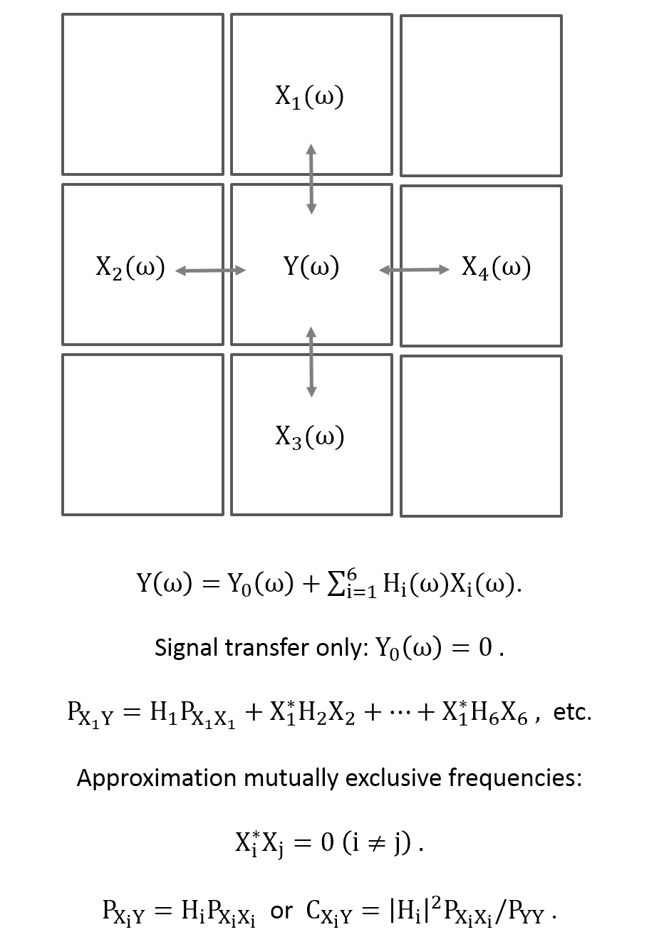
Figure 1: Schematics of the local signal propagation model. The center voxel with signal y(t) is described by a linear model of its nearest neighbor signals in frequency space. The model is called a signal propagation or transfer model because the contribution of the center voxel itself is not taken into account, only the signals exchanged between voxels. Further assumptions are provided in the equations.
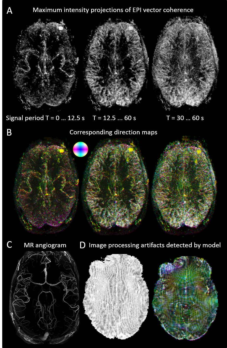
Figure 2: Local signal transfer estimated from EPI data (A, B), and angiogram of the same data set (C). Artifacts after application to standard pre-processed data, picking up effects of signal re-sampling and distortion correction (D).
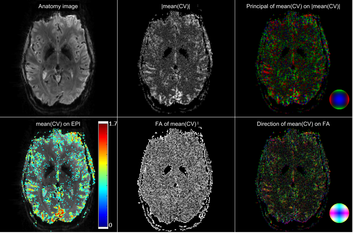
Figure 3: Coherence vector (CV) maps for one slice. The CV depends on frequency, and mean(CV) is the average CV over frequencies from 0.017 to 0.033 Hz (periods of 30 to 60 s). FA = fractional anisotropy, computed from the principal CV component.