0063

Simultaneous Magnetic Resonance Angiography and Multiparametric Mapping in the Transient-state

Pedro A Gomez^1,2, Miguel Molina-Romero^1,2, Guido Buonincontri³, Bjoern H Menze¹, and Marion I Menzel²

¹Technical University of Munich, Munich, Germany, ²GE Global Research, Munich, Germany, ³Imago7 Foundation, Pisa, Italy

Synopsis

Quantitative Transient-state Imaging (QTI) is a non-random, dictionary-less MR Fingerprinting alternative. Through iterative reconstructions, QTI recovers a series of contrast-weighted images from transient-state acquisitions and subsequently estimates the parameters that best describe the resulting dynamic signal evolutions. Here, we extend the QTI framework by incorporating a simple velocity model that accounts for blood flowing into and out of the imaging slice. The model, however wrong, can be very useful: it predicts signal hyperintensities in the presence of flow, allowing for the simultaneous reconstruction of MR Angiography images, hundreds of dynamic contrast-weighted images, and their corresponding parametric maps.

Introduction

Multiparametric mapping methods, such as Quantitative Transient-state Imaging (QTI)[1] and MR Fingerprinting (MRF)[2], enable the estimation of several parametric maps with a single acquisition by enforcing consistency with a model. If such model is assumed to be perfect, the estimated parametric maps contain all the relevant information. However, commonly used models have limitations, and by consequence the maps can disregard useful information.

Here, we propose to simultaneously reconstruct images and compute parametric maps, and demonstrate that simple models, however wrong, can be very useful in the context of contrast-weighted imaging. For example, by accounting for blood flowing through an imaging slice with a mean velocity scalar, we can predict a signal hyperintensity throughout the course of the acquisition. Thus, the reconstructed signals can be taken advantage of to obtain MR Angiography (MRA) images.

Methods

In the transient-state, the observed signal over time $$$y(t)\in\mathbb{C}^T$$$ with $$$T$$$ measurements can be described as a spatial function modulated by a temporal signal:

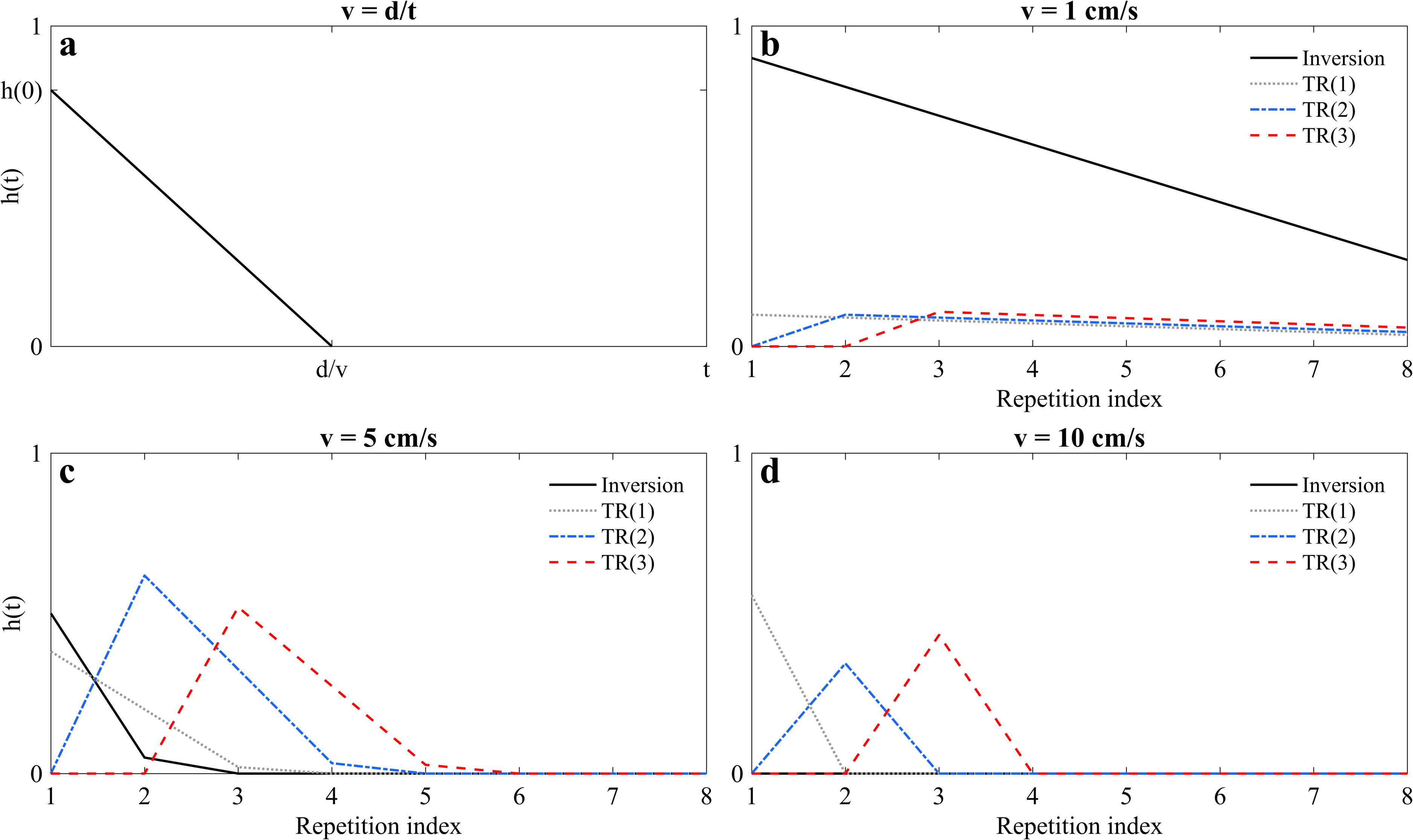
$$y(t)=\int_\mathbf{r}\rho(\mathbf{r})f_t(\mathbf{r})e^{-2\pi i\mathbf{k}(t)\cdot\mathbf{r}}d\mathbf{r};$$ where $$$\rho(\mathbf{r})$$$ is the spin density at position $$$\mathbf{r}$$$, $$$\mathbf{k}(t)$$$ is the $$$k$$$-space trajectory, and $$$f_t(\mathbf{r})$$$ is the temporal signal, given by the recursion: $$f_t(\mathbf{r})=\sum_{i=0}^Tf_{i-1}f_t(\mathbf{r})g\left(\eta_i;\theta(\mathbf{r})\right)\ast h_i(t).$$ The signal $$$f_t (\mathbf{r})$$$ is determined at sample time $$$i$$$ by an operation $$$g\left(\cdot \right)$$$ on the signal from the previous sample $$$f_{i-1}(\mathbf{r})$$$, where the operator $$$g\left(\cdot \right)$$$ is a function of two parameter sets: the temporally varying acquisition parameters $$$\eta_i$$$, and the spatially dependent biophysical parameters of interest, such as T1$$$(\mathbf{r})$$$ and T2$$$(\mathbf{r})$$$. Finally, $$$h_i(t)$$$ gives the fraction of spins tagged with RF pulse $$$i$$$ that will remain in the imaging slice after time $$$t$$$. We have chosen $$$h(t)$$$ as plug flow (Fig. 1), i.e. a constant velocity scalar over time[3].

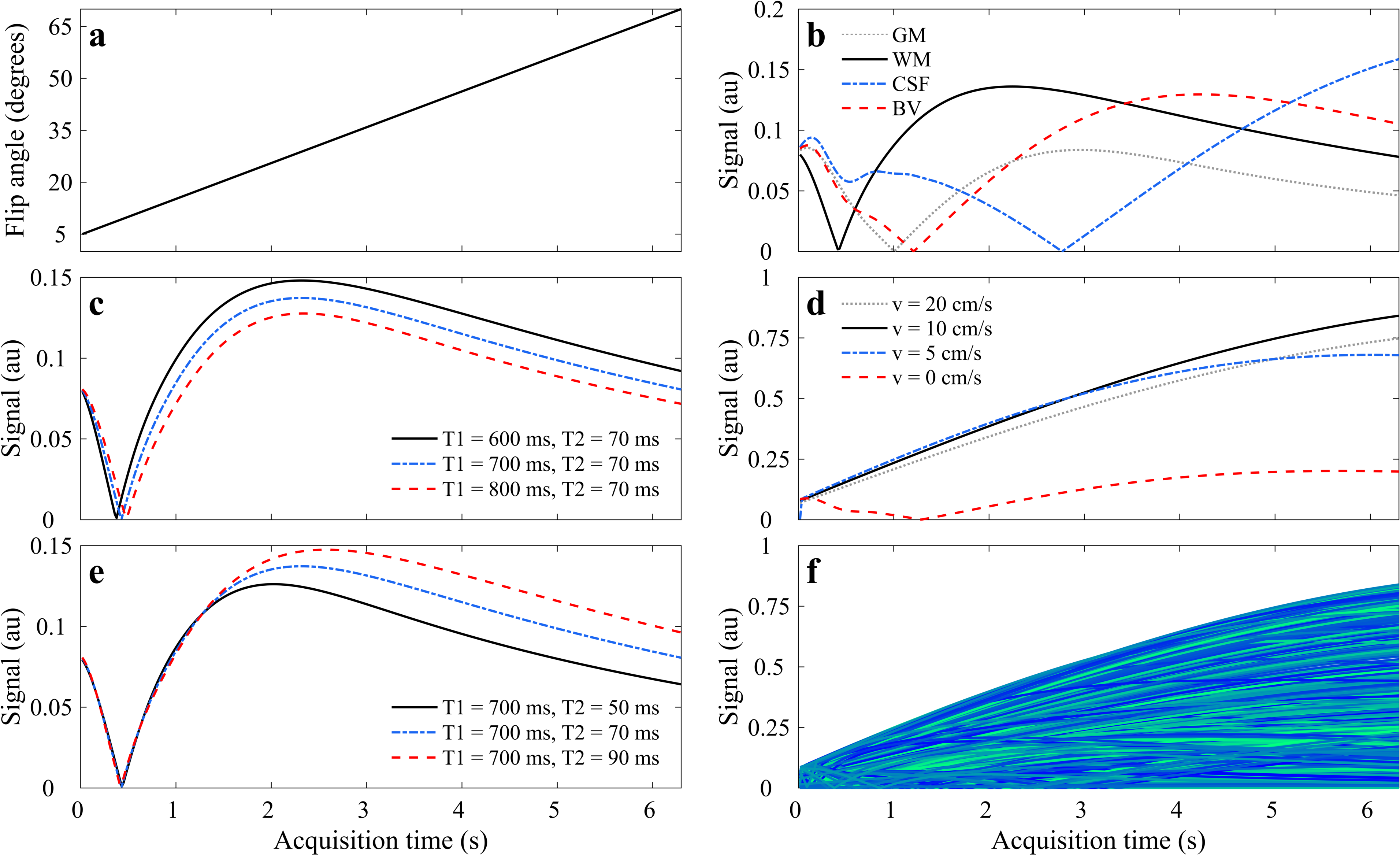
Although flow is not constant in time or across the lumen of a vessel, modeling it as a constant scalar predicts the presence of unsaturated spins with every RF pulse. These spins will cause signal hyperintensities in the transient-state, whereas stationary spins will become saturated and follow the dynamics dictated by the choice of acquisition parameters $$$\eta_i$$$ (Fig. 2).

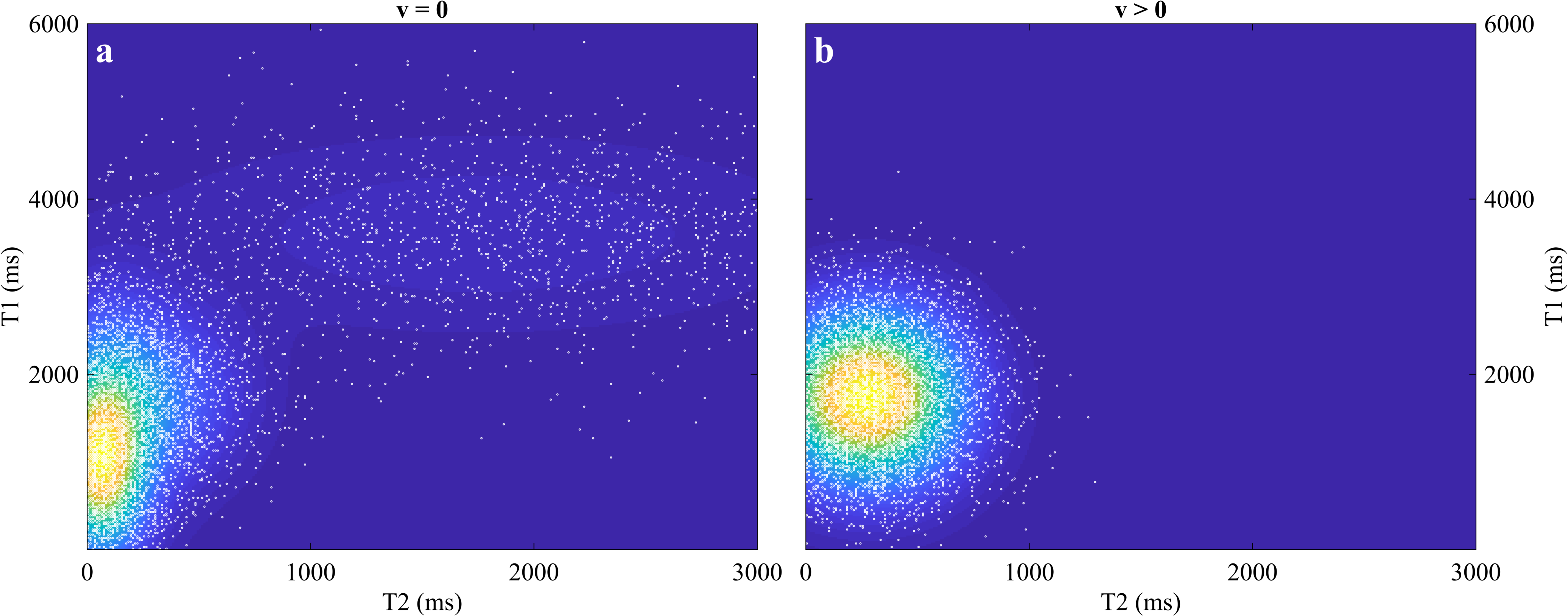
We acquired 112, 2 mm thick slices of a healthy volunteer on a GE 3T MR750w scanner with a 12 channel receive only head RF coil (GE Medical Systems, Milwaukee, WI). For every slice, we inverted the magnetization locally and then applied a train of 350 RF pulses with a flip angle ramp described in Fig. 2a and TR/TE = 18/2 ms. In every repetition, we acquired data with a variable density spiral with 1 mm in-plane resolution. We reconstructed the entire four-dimensional dataset using the reconstruction proposed in[1], where we projected the data onto a lower dimensional temporal subspace[4] and regularized the reconstruction with a local low-rank operation on 4D spatiotemporal image patches. We created the subspace by sampling a prior distribution of tissue classes for both stationary and non-stationary tissues (Fig. 3 and Fig. 2f), and simulated the signal over time using the EPG formalism[5]. After reconstruction, we estimated T1, T2, and proton density (PD) from the temporal dynamics and summed all temporal frames into one volume to create MRA images.

Results

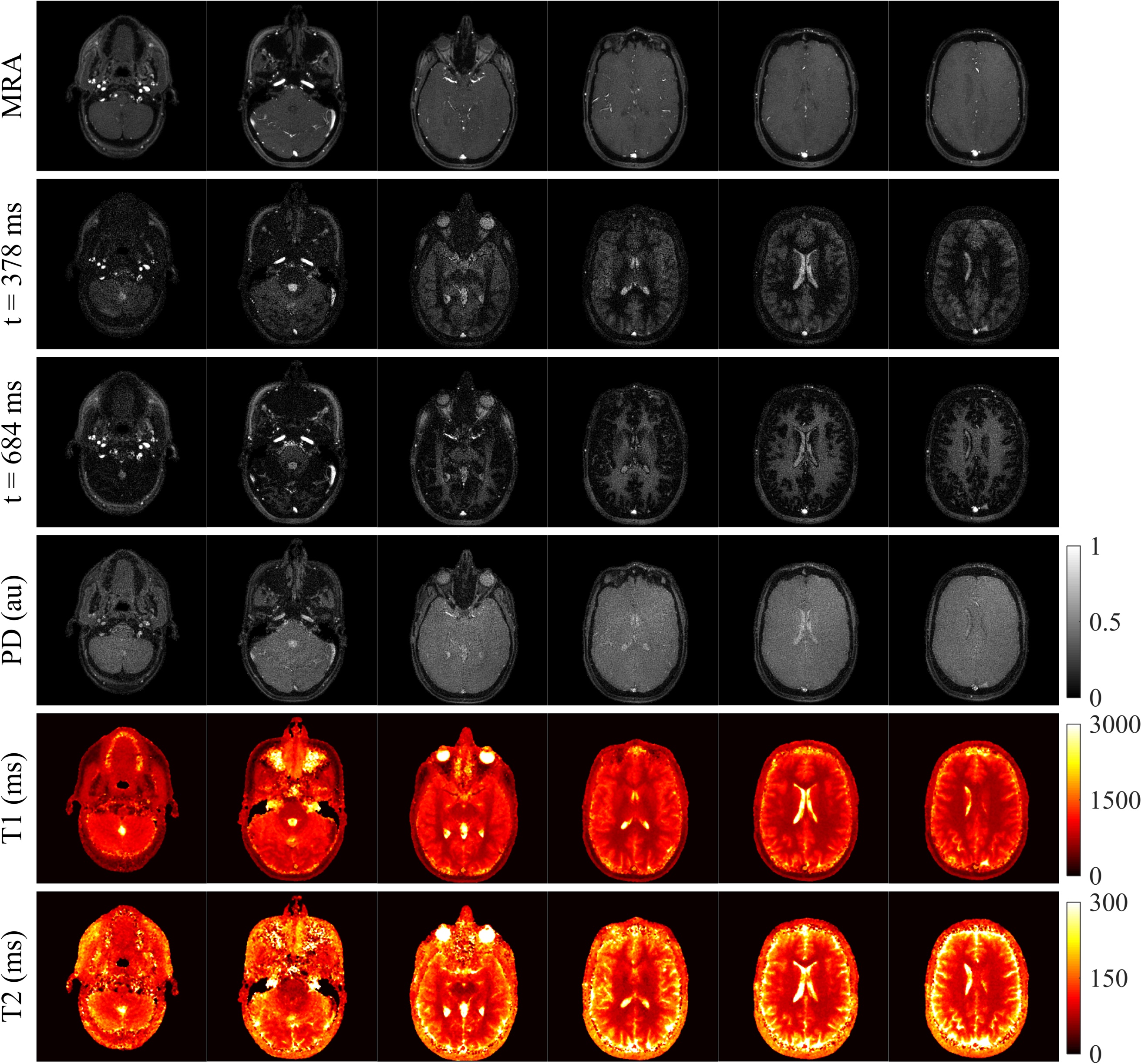
Figure 4 shows several slices of the obtained MRA images, contrast-weighted images at different points in time, and their resultant parametric maps. The MRA images give anatomical context of the location of veins and arteries inside and around the brain. The contrast-weighted images provide unique contrasts and are informative on the T1 and T2 times of different tissues. For example, at $$$t=378$$$ ms, white matter is close to its inversion time, whereas gray matter has not yet inverted; at $$$t=684$$$ ms, contrast is reversed as gray matter reaches its inversion while white matter recovers signal and is still not affected by T2 relaxation. The estimated parametric maps are consistent with previous literature findings[6]–[12]. Figure 5 displays a maximum intensity projection of the MRA images, where important structures such as the circle of Willis, the carotid arteries, and the superior sagittal sinus can be identified. Pulsatile artifacts on the slices, especially in the neck region, can also be observed.

Discussion

By acquiring thin axial slices, we were able to make use of time-of-flight effects in the transient-state to recover MRA images. While our model relies on a velocity scalar that oversimplifies the complex reality of blood flow inside vessels, it still enables us to create MRA images that could have significant diagnostic value.

Conclusion

We demonstrated an extension to QTI that allows for the reconstruction of MRA images, multiple contrast-weighted images, and parametric maps from the same scan.

Acknowledgements

With the support of the TUM Institute for Advanced Study, funded by the German Excellence Initiative and the European Commission under Grant Agreement Number 605162.

References

[1] P. A. Gómez, G. Buonincontri, M. Molina-Romero, J. I. Sperl, M. I. Menzel, and B. H. Menze, “Accelerated parameter mapping with compressed sensing: an alternative to MR Fingerprinting,” Proc Intl Soc Mag Reson Med, 2017.

[2] D. Ma, V. Gulani, N. Seiberlich, K. Liu, J. L. Sunshine, J. L. Duerk, and M. A. Griswold, “Magnetic resonance fingerprinting,” Nature, vol. 495, pp. 187–192, 2013.

[3] L. Axel, “Blood flow effects in magnetic resonance imaging,” Am.J.Roentgeno., vol. 143, pp. 1157–1166, 1984.

[4] J. I. Tamir, M. Uecker, W. Chen, P. Lai, M. T. Alley, S. S. Vasanawala, and M. Lustig, “T2 shuffling: Sharp, multicontrast, volumetric fast spin-echo imaging,” Magn. Reson. Med., 2016. [

5] M. Weigel, “Extended phase graphs: Dephasing, RF pulses, and echoes - pure and simple,” J. Magn. Reson. Imaging, 2014.

[6] H. Lu, L. M. Nagae-Poetscher, X. Golay, D. Lin, M. Pomper, and P. C. M. Van Zijl, “Routine clinical brain MRI sequences for use at 3.0 tesla,” J. Magn. Reson. Imaging, vol. 22, no. 1, pp. 13–22, 2005.

[7] T. Ethofer, I. Mader, U. Seeger, G. Helms, M. Erb, W. Grodd, A. Ludolph, and U. Klose, “Comparison of Longitudinal Metabolite Relaxation Times in Different Regions of the Human Brain at 1.5 and 3 Tesla,” Magn. Reson. Med., vol. 50, no. 6, pp. 1296–1301, 2003.

[8] N. Gelman, J. M. Gorell, P. B. Barker, R. M. Savage, E. M. Spickler, J. P. Windham, and R. A. Knight, “MR Imaging of Human Brain at 3.0 T: Preliminary Report on Transverse Relaxation Rates and Relation to Estimated Iron Content,” Radiology, vol. 210, no. 3, pp. 759–767, 1999.

[9] A. MacKay, C. Laule, I. Vavasour, T. Bjarnason, S. Kolind, and B. Mädler, “Insights into brain microstructure from the T2 distribution,” Magn. Reson. Imaging, vol. 24, no. 4, pp. 515–525, 2006.

[10] S. A. Smith, R. A. E. Edden, J. A. D. Farrell, P. B. Barker, and P. C. M. Van Zijl, “Measurement of T1 and T2 in the cervical spinal cord at 3 Tesla,” Magn. Reson. Med., vol. 60, no. 1, pp. 213–219, 2008.

[11] K. P. Whittall, A. L. Mackay, D. A. Graeb, R. A. Nugent, D. K. B. Li, and D. W. Paty, “In vivo measurement ofT2 distributions and water contents in normal human brain,” Magn. Reson. Med., vol. 37, no. 1, pp. 34–43, 1997.

[12] R. Noeske, F. Seifert, K. H. Rhein, and H. Rinneberg, “Human cardiac imaging at 3 T using phased array coils.,” Magn. Reson. Med., vol. 44, no. 6, pp. 978–82, 2000.

Figures

Figure 1: Plug flow and washout from an imaging slice. a, Fraction of spins $$$h(t)$$$ remaining in a slice after being tagged by an RF pulse at $$$h(0)$$$, where $$$d$$$ is the slice thickness and $$$v$$$ is the mean velocity. b-d, The total number of repetitions that spins tagged by a certain pulse remain in the slice is proportional to their velocity, where spins flowing slowly will remain in the slice longer than faster spins. Furthermore, the starting fraction of fresh spins in a subsequent RF pulse is equivalent to the fraction of spins that have washed out from the previous pulse.

Figure 2: Acquisition scheme and signal modeling. a, Flip angle trajectory, where an inversion pulse followed by a linear flip angle ramp provides T1 encoding (c) at different inversion times and T2 encoding from stimulated echoes at higher flip angles (e). b, Signal evolution for four distinct tissue classes, gray matter (GM), white matter (WM), cerebrospinal fluid (CSF), and stationary blood (BV). d, In the presence of flow, there will be unsaturated magnetization in every repetition, producing signal hyperintensities. f, An ensemble of simulated stationary and flowing signal evolutions can be taken advantage of to recover the temporal signal dynamics for every voxel in the image.

Figure 3: Prior sampling. a, Four stationary tissue classes (WM, GM, CSF, and BV) were considered, where the ranges of each tissue class were informed from literature[6]–[12]. We used the following ranges: WM 661-1155/52-72 ms; GM 945-1934/61-106 ms; CSF 3200-4000/1000-2500; BV 1465-2020/225-325. b, In the non-stationary case, only the BV prior was taken into account. Velocity was sampled evenly from 0 cm/s to 100 cm/s, which is the upper bound for spins remaining in the slice with an echo time of 2 ms and a slice thickness of 2 mm.

Figure 4: Simultaneous MRA, contrast-weighted imaging, and parametric mapping. Accounting for flow effects allows for the simultaneous reconstruction of MRA images, as many contrast-weighted images as repetitions in the sequence, and the related parametric maps.

Figure 5: 3D maximum intensity projection of MRA data. The MRA volume was obtained by summing all of the frames in the transient-state acquisition. Thereafter, a 3D maximum intensity projection results in the visualization of all of the main vascular structures in the head.

Proc. Intl. Soc. Mag. Reson. Med. 26 (2018)

0063