0061
Silent, 3D MR Parameter Mapping using Magnetization Prepared Zero TE1ASL Europe, GE Healthcare, Munich, Germany, 2Neuroimaging, King’s College London, London, United Kingdom
Synopsis
Here we describe a novel method for 3D, quantitative, silent MR parameter mapping based on 1) combined T1 and T2 magnetization preparation, 2) Zero TE image encoding and 3) least-squares dictionary matching.
Introduction
Zero TE1-4 provides efficient, fast and robust 3D radial image encoding. This is because of its negligibly short RF pulses (i.e. RF pulse width ≤ (Imaging Bandwidth)-1), short repetition times (i.e. TR ~ number of readout points*sampling time) and high sampling efficiency (most of the repetition time used for data acquisition). Furthermore, it allows silent imaging (due to minimal gradient switching) and is robust against motion (3D radial) and off-resonance (TE=0).Because of the low flip angles used, Zero TE results in native proton density (PD) contrast with minimal T1 saturation3-5. Magnetization preparation, like Inversion Recovery (IR) and T2 preparation, has been used for T1-, or T2-weighted anatomical and functional imaging6-9. The efficient, robust and silent imaging performance renders Zero TE perfectly suited for the spatial encoding of magnetization prepared longitudinal magnetization.
Here we describe a novel method for 3D, quantitative, silent MR parameter mapping based on 1) combined T1 and T2 magnetization preparation, 2) Zero TE image encoding and 3) least-squares dictionary matching.
Methods
Figure
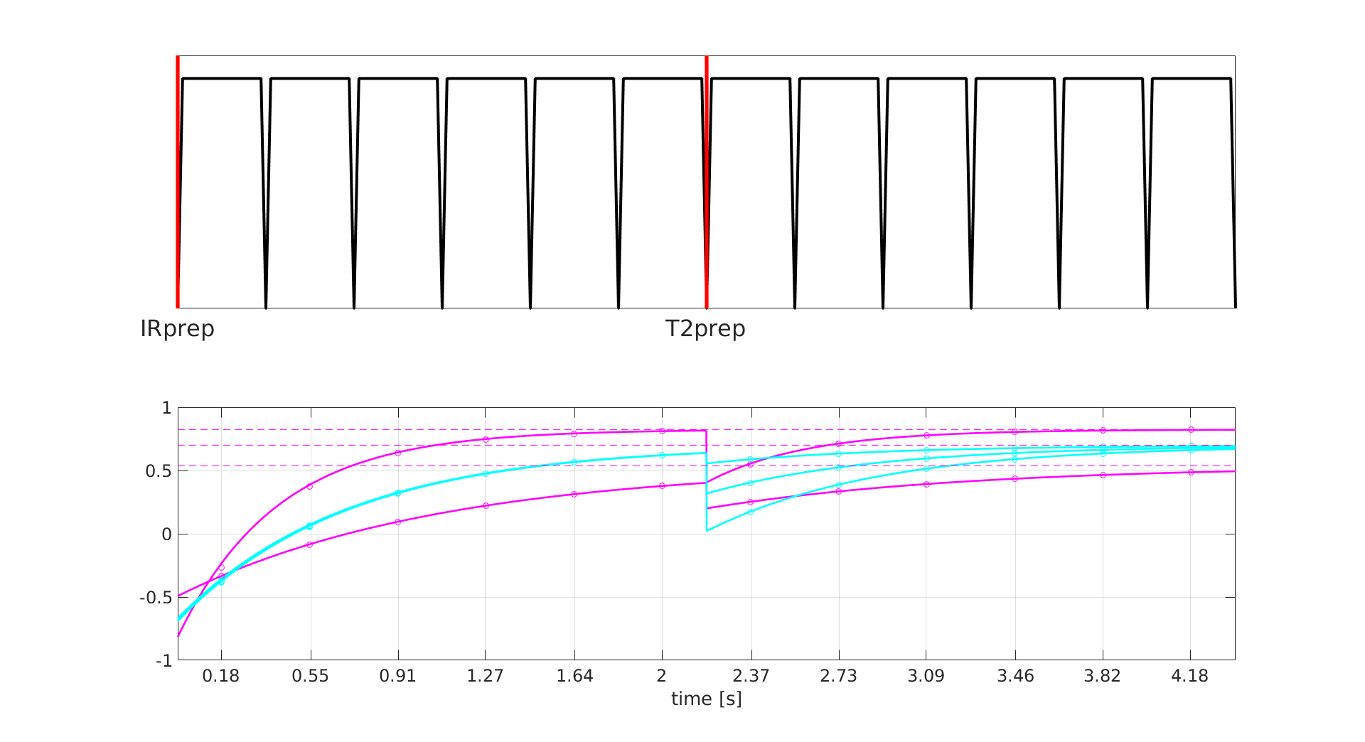
1 illustrates the pulse sequence, starting with 1) IR preparation followed by
2) six Zero TE readout segments, followed by 3) T2 preparation, followed by 4) another
six Zero TE readout segments. Each Zero TE
readout module, consists of NSpkSeg=256 radial spokes per segment. The sequence is repeated (total number of
spokes / NSpkSeg=96 times) for full 3D spatial
encoding.
The
evolution of an initial longitudinal magnetization (Mz,0) following
a Zero TE readout of n repetitions with flip angle α and repetition time TR can be
stated as:
Mz,n
= Mz,0 E1n cosnα + M0
(1- E1) (1- E1n cosnα)
/ (1- E1 cosα)
with
M0 the thermal equilibrium magnetization (i.e. proton density), and E1
= e-TR/T1, assuming perfect spoiling of transverse magnetization for
each TR. Perfect magnetization
preparation was assumed for both inversion recovery (i.e. Mz,n -> -1.0*Mz,n) and T2
preparation (i.e. Mz,n -> e-TE/T2*Mz,n). The twelve Zero TE signals can be modeled as the
average of Mz,n over the corresponding NSpkSeg spokes per
segment (cf. Figure 1).
Quantitative
PD, T1 and T2 parameter maps were obtained via pixel-wise, least-squares
matching of the measured Zero TE signals (Measurem) to the
dictionary of modeled Zero TE signals (Modelm(T1,T2)):
Minimize: ∑m | Measurem(r)
– PD(T1,T2)*Modelm(T1,T2) |2, with
PD=∑m(Measurem(r)*Modelm)/∑m(Modelm*Modelm).
The
dictionary was calculated for a 384x384 equidistant grid of T1 (0.2s to 7s) and
T2 (0.01s to 1.5s) values.
The magnetization
prepared Zero TE sequence (Figure 1) was implemented on a 3T MR750w scanner (GE
Healthcare, Chicago, IL, USA) and tested in a T1/T2 phantom10
and healthy volunteers. Preparation was performed with adiabatic tanh/tan inversion and numerically
optimized T2 preparation designed to be robust against ±40% B1 variation and
±250Hz B0 off-resonance9. Zero TE imaging parameters
were set to FOV=192mm, 1.5mm isotropic resolution, BW=±31.25kHz, FA=2°,
TR=1.4ms per spoke, 24576 total spokes per image, NSpkSeg=256 spokes
per segment, scan time ~7min. Data
processing, including 3D gridding image reconstruction, least-squares
dictionary matching and visualization was done using Matlab (Mathworks, Natick,
MA).
Results
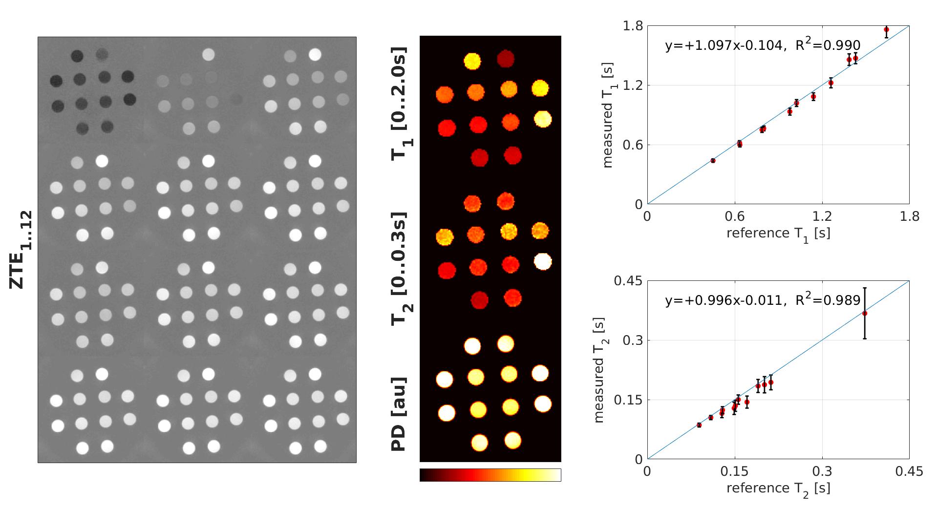
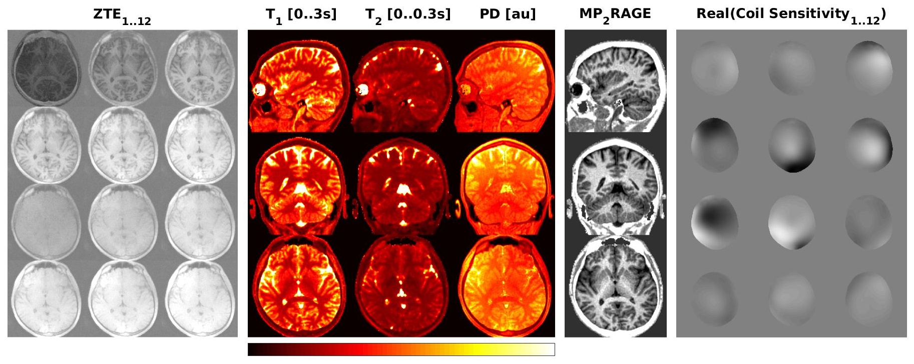
Figure 2 illustrates results for the Eurospin T05 phantom10 containing tubes of known T1 and T2 relaxation time. The left subplot shows the twelve Zero TE images in axial orientation used as input (Measurem(r)) for the least-squares dictionary matching. The middle subplot illustrates derived PD, T1 and T2 parameter maps. The right subplot compares measured versus reference T1 and T2 values with an excellent R2=0.99. Figure 3 illustrates corresponding in-vivo head results obtained in a healthy volunteer. An MP2RAGE11-type image was derived as well (i.e. 2nd Zero TE image (TI~395ms), normalized by the fitted PD) which can be used for anatomical inspection. The MP2RAGE image demonstrates excellent white matter, gray matter, CSF contrast and is clean of spatial RF bias. Furthermore, the obtained 3D radial images permit auto-calibrated coil sensitivity calibration (right). The in-bore acoustic noise of the sequence was measured to be only ~5dBA above ambient noise; primarily originating from the gradient spoiler following the preparation pulses. The sampling efficiency was measured to be ~75%.Discussion and Conclusion
The presented magnetization prepared Zero TE pulse sequence allows quantitative, 3D, silent parameter mapping. The preparation pulses fan out the Mz magnetization along the T1 and T2 contrast dimension which subsequently gets spatially encoded using Zero TE. Compared to gradient-echo, or spin-echo encoding, Zero TE is faster (TR~1.4ms) with favorably high sampling efficiency, more robust against motion and off-resonance, and silent. The measured Zero TE images can be decomposed into constituent PD, T1 and T2 MR parameters maps using least-squares dictionary matching (cf. Figures 2, 3). Alternatively, the Zero TE images can also be used for standard MP2RAGE-type anatomical imaging.Acknowledgements
No acknowledgement found.References
[1] Madio et al. "Ultra‐fast imaging using low flip angles and fids." Magnetic resonance in medicine 34.4 (1995): 525-529.[2] Wu et al. "Density of organic matrix of native mineralized bone measured by water‐and fat‐suppressed proton projection MRI." Magnetic resonance in medicine 50.1 (2003): 59-68. [3] Weiger et al. "MRI with zero echo time: hard versus sweep pulse excitation." Magnetic resonance in medicine 66.2 (2011): 379-389. [4] Grodzki et al. "Ultrashort echo time imaging using pointwise encoding time reduction with radial acquisition (PETRA)." Magnetic resonance in medicine 67.2 (2012): 510-518.[5] Wiesinger, Florian, et al. "Zero TE MR bone imaging in the head." Magnetic resonance in medicine 75.1 (2016): 107-114. [6] Alibek et al. "Acoustic noise reduction in MRI using Silent Scan: an initial experience." Diagnostic and Interventional Radiology 20.4 (2014): 360.[7] Ida et al. "Quiet T1‐weighted imaging using PETRA: Initial clinical evaluation in intracranial tumor patients." Journal of Magnetic Resonance Imaging 41.2 (2015): 447-453. [8] Solana et al. "Quiet and distortion‐free, whole brain BOLD fMRI using T2‐prepared RUFIS." Magnetic resonance in medicine 75.4 (2016): 1402-1412. [9] Janich et al. “Optimal control B1-robust T2 preparation”. ISMRM 2017: 391. [10] Lerski et al. "II. Performance assessment and quality control in MRI by Eurospin test objects and protocols." Magnetic resonance imaging 11.6 (1993): 817-833. [11] Marques et al. "MP2RAGE, a self bias-field corrected sequence for improved segmentation and T 1-mapping at high field." Neuroimage 49.2 (2010): 1271-1281.
Figures