0030
Portable single-sided MR: multicomponent T2 relaxometry and depth profiling with a Unilateral Linear Halbach sensor1Electrical Engineering & Computer Science, Massachusetts Institute of Technology, Cambridge, MA, United States, 2David H. Koch Institute For Integrative Cancer Research, Massachusetts Institute of Technology, Cambridge, MA, United States, 3A. A. Martinos Center for Biomedical Imaging, Massachusetts General Hospital, Charlestown, MA, United States, 4Harvard Medical School, Boston, MA, United States, 5Department of Materials Science and Engineering, Massachusetts Institute of Technology, Cambridge, MA, United States
Synopsis
Widely accessible, fast, and portable MR relaxometry can provide highly valuable diagnostic information in many diseases including fluid overload, dehydration, and muscle degeneration. High cost, large size, and extended acquisition time limit the use of traditional MRI for relaxometry.
We introduce a novel portable MR sensor with a large, remote, uniform magnetic field created by a Unilateral Linear Halbach array capable of performing spatially selective, multi-component relaxometry.
Strong agreement between simulation and experimental results indicates highly reliable magnet design methods. Spatial selectivity is achieved through variation of either RF pulse length or B1 frequency. Quantitative multi-component T2 relaxometry is demonstrated.
Background and Purpose
Magnetic resonance (MR) relaxometry provides a unique diagnostic biomarker capable of identifying and evaluating many diseases including fluid overload (congestion), dehydration, tendon injuries, traumatic brain injury, breast cancer, and muscle degeneration1–8.
High cost, resource intensiveness, large size, and extended acquisition time limit the accessibility of MR relaxometry to a small subset of patients9. Further, MRI is not well suited for the very fast (TE < 1ms) and long echo trains (>2000) required by high resolution relaxometry10. Portable MR ameliorates many of these limitations, but low penetration depth and sensitivity often limit their medical utility11–13.
We introduce a novel portable MR sensor (Figures 1 & 2), based on the previously reported Unilateral Linear Halbach magnet design14. This sensor utilizes a large, remote, uniform magnetic field to perform spatially selective (Figures 3 & 4) multi-component relaxometry (Figure 5). The large volume of the uniform region and optimized RF coil geometry provide the ability to perform high sensitivity MR measurements with short acquisition times enabling precise quantitative resolution of multiple T2 compartments.
Methods and Results
Unilateral Linear Halbach magnet design and construction
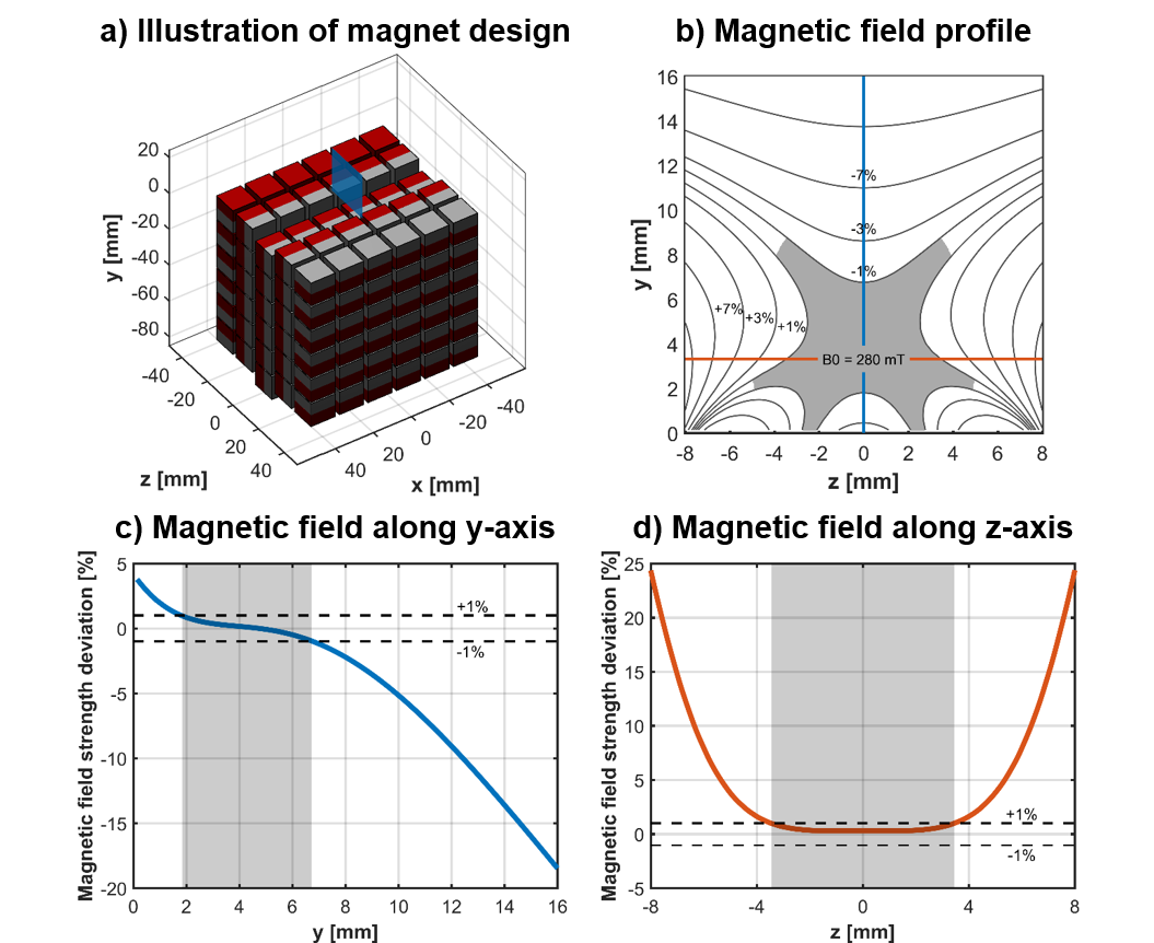
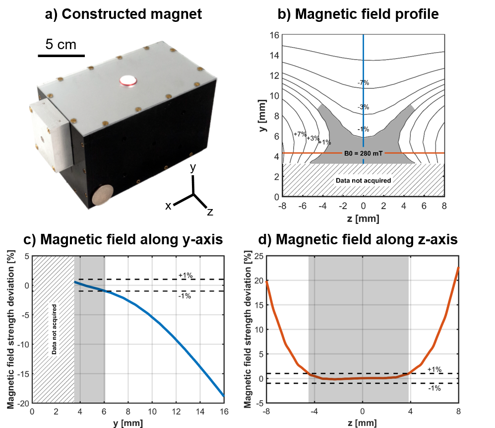
Design methods and guidelines previously described were utilized to create a magnet assembly with the following properties: uniform region volume > 500 mm3, field strength > 0.25 Tesla, measurement depth ~4 mm, and magnet volume < 600 cm3 (Figures 1a & 2a).
Finite element analysis with COMSOL Multiphysics (Burlington, MA) was performed to evaluate the magnetic field created by the permanent magnet assembly. The uniform region of the magnetic field was defined as a region spanning the RF pulse bandwidth (~1%) with orientation horizontal to the surface of the magnet (Figures 1b & 2b). The sweet spot of the uniform region is formed by a saddle region (Figures 1c-d & 2c-d). The shape of the magnetic field of the constructed magnet very closely matched simulation results (Figure 2b-d).
RF pulse length and spin echo bandwidth
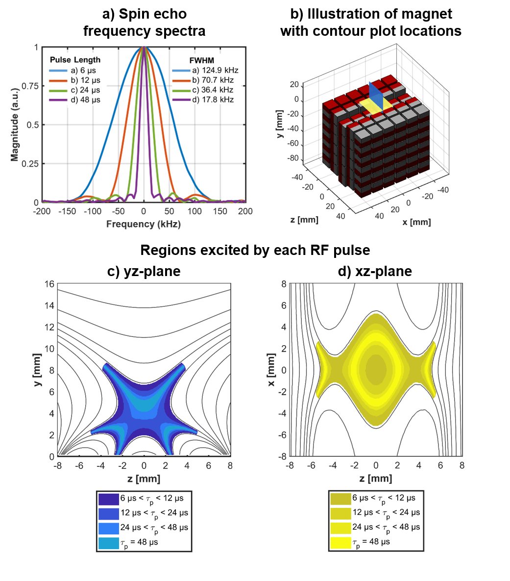
The dimensions of the RF transceiver coil were optimized for signal strength. The duration of the excitation and refocusing pulses were varied and the effect on the spin echo bandwidth characterized (Figure 3a). The FWHM bandwidth varied inversely with the pulse length indicating that a shorter pulse is able to excite a larger fraction of the uniform region. Results of a simulation of the excited volume at various RF pulse lengths, given the measured echo bandwidths, indicate that shorter pulses excite larger and more contiguous regions (Figure 3c-d).
Depth profiling with planar sample
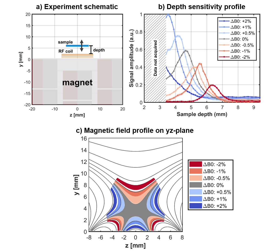
The sensitive region is located distal to the surface of the magnet and its location can be controlled by varying B1 frequency. By taking advantage of this field profile, measurements can be performed selectively on deep structures without interference from shallower tissue. A thin (800 μm) planar sample of 40 mM aqueous paramagnetic copper sulfate solution was prepared15. The sample was oriented parallel to the surface of the magnet (xz-plane) and measured at various distances (depths) away from the surface of the sensor (CPMG, TE 65 us, NE 2000, 1 MHz acquisition bandwidth, pulse length 12 μs). The amplitude of the signal from the sample varied with depth with a peak occurring at the sweet spot of the uniform region (Figure 4). By varying the B1 frequency, the profile shape and location can be tuned.
Multi component T2 relaxometry
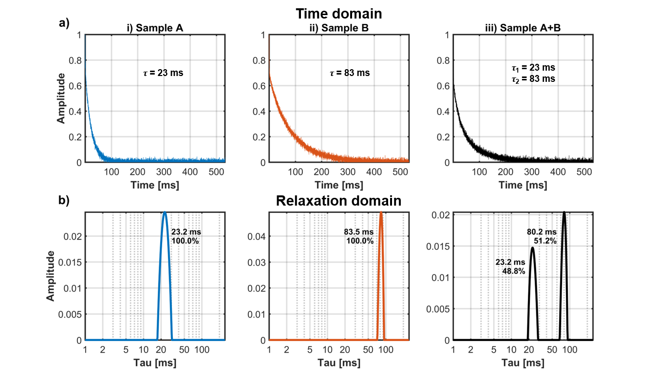
Phantoms consisting of glass capillary tubes filled with aqueous copper sulfate at i) 40 mM, ii) 10 mM, and iii) 50% 40 mM and 50% 10 mM were measured (CPMG, TE 65 us, NE 8192, 1 MHz acquisition bandwidth) (Figure 5a). CPMG decay curves were transformed into relaxation domain spectra using the inverse Laplace transform (Figure 5b)16,17. The sensor is able to resolve the decay rates and amplitudes of samples with multiple relaxation peaks to within 4% accuracy (Figure 5b).
Discussion and Conclusion
The Unilateral Linear Halbach sensor is capable of performing multi component T2 relaxometry with spatial selectivity. The ability to interrogate anatomical structures beyond the surface of the body is critical to realizing the diagnostic value of portable T2 relaxometry. The sensor can be tuned for maximal sensitivity at a depth that allows substantial tissue penetration. This tunable sensitivity suggests the potential to resolve structures with sub-mm spatial resolution perpendicular to the magnet surface.
Future work will explore the diagnostic utility of portable MR relaxometry, beginning with disorders in fluid regulation. Shaped RF pulses could expand the sensitive region without exceeding RF exposure limits. Precise control over excitation and inversion pulse bandwidth would allow more accurate depth profiling. Shaped pulses, such as hyperbolic secant and WURST, have demonstrated strong frequency selectivity and robustness to field inhomogeneity18,19.
Acknowledgements
Funding from MIT Institute for Soldier Nanotechnologies (United States Army Research Office Grant W911NF-13D-0001), National Institutes of Health – National Cancer Institute Centers of Cancer Nanotechnology Excellence Grant U54 CA151884-02, a Hertz Foundation Fellowship, and a National Science Foundation Graduate Fellowship.References
1. Shenton, M. E. et al. A review of magnetic resonance imaging and diffusion tensor imaging findings in mild traumatic brain injury. Brain Imaging Behav. 6, 137–192 (2012).
2. Warakaulle, D. R. & Anslow, P. Differential diagnosis of intracranial lesions with high signal on T1 or low signal on T2-weighted MRI. Clin. Radiol. 58, 922–933 (2003).
3. Chaudhari, A. S. et al. Imaging and T2 relaxometry of short‐T2 connective tissues in the knee using ultrashort echo‐time double‐echo steady‐state (UTEDESS). Magn. Reson. Med. (2017).
4. Lehman, C. D. & Schnall, M. D. Imaging in breast cancer: magnetic resonance imaging. Breast Cancer Res. 7, 215 (2005).
5. Polak, J. F., Jolesz, F. A. & Adams, D. F. Magnetic Resonance Imaging of Skeletal Muscle Prolongation of T1 and T2 Subsequent to Denervation. Invest. Radiol. 23, 365–369 (1988).
6. Theodorou, D. J., Theodorou, S. J. & Kakitsubata, Y. Skeletal muscle disease: patterns of MRI appearances. Br. J. Radiol. 85, e1298–e1308 (2012).
7. Li, M., Vassiliou, C. C., Colucci, L. A. & Cima, M. J. (1)H nuclear magnetic resonance (NMR) as a tool to measure dehydration in mice. NMR Biomed. 28, 1031–9 (2015).
8. Kodibagkar, V. D., Cui, W., Merritt, M. E. & Mason, R. P. Novel 1H NMR approach to quantitative tissue oximetry using hexamethyldisiloxane. Magn. Reson. Med. 55, 743–748 (2006).
9. Carneiro, A. A. O., Vilela, G. R., de Araujo, D. B. & Baffa, O. MRI relaxometry: methods and applications. Brazilian J. Phys. 36, 9–15 (2006).
10. Pell, G. S. et al. Optimized clinical T2 relaxometry with a standard CPMG sequence. J. Magn. Reson. Imaging 23, 248–252 (2006).
11. Haken, R. & Blümich, B. Anisotropy in tendon investigated in vivo by a portable NMR scanner, the NMR-MOUSE. J. Magn. Reson. 144, 195–199 (2000).
12. Casanova, F., Perlo, J. & Blümich, B. Single-sided NMR. Single-Sided NMR (Springer Berlin Heidelberg, 2011). doi:10.1007/978-3-642-16307-4
13. Hansen, P. C. & O’Leary, D. P. The use of the L-curve in the regularization of discrete ill-posed problems. SIAM J. Sci. Comput. 14, 1487–1503 (1993).
14. Bashyam, A., Li, M. & Cima, M. J. Unilateral Linear Halbach magnets for single sided NMR: Generalized design framework and experimental validation. in Proceedings of the International Society for Magnetic Resonance in Medicine 2017 Annual Meeting (2017).
15. Barnhart, J. L. & Berk, R. N. Influence of paramagnetic ions and pH on proton NMR relaxation of biologic fluids. Invest. Radiol. 21, 132–136 (1986).
16. Bai, R., Koay, C. G., Hutchinson, E. & Basser, P. J. A framework for accurate determination of the T2 distribution from multiple echo magnitude MRI images. J. Magn. Reson. 244, 53–63 (2014).
17. Grant, M., Boyd, S. & Ye, Y. CVX: Matlab software for disciplined convex programming. (2008).
18. Stockmann, J. P., Cooley, C. Z., Guerin, B., Rosen, M. S. & Wald, L. L. Transmit Array Spatial Encoding (TRASE) using broadband WURST pulses for RF spatial encoding in inhomogeneous B 0 fields. J. Magn. Reson. 268, 36–48 (2016).
19. Park, J. & Garwood, M. Spin‐echo MRI using π/2 and π hyperbolic secant pulses. Magn. Reson. Med. 61, 175–187 (2009).
Figures