MSK Applications of Diffusion Weighted Imaging: Technical Aspects
1NYU School of Medicine
Synopsis
The objective of this talk is to present a hands-on on the acquisition and processing of diffusion-weighted imaging tailored to MSK applications. In this presentation we will
explain how diffusion is measured and which is the meaning of the experimental parameters;-
discuss the different acquisition strategies for diffusion-weighted imaging; and learn how to optimize a diffusion protocol for a given
Objectives
The objective of this talk is to present a hands-on on the acquisition and processing of diffusion-weighted imaging tailored to MSK applications. In this presentation you will:
1. Understand how diffusion is measured and which is the meaning of the experimental parameters diffusion time, pulse duration, diffusion direction and diffusion weighting...
2. Know the different acquisition strategies for diffusion-weighted imaging
3. Learn how to optimize a diffusion protocol for a given
General ideas about diffusion
In tissue non-bounded small ions and molecules displace through the extracellular matrix as a consequence of their thermal energy. In its motion small molecules collide with the solid extracellular matrix found in its pathway (collagen fibers, cell membranes…). The process of how the molecules spread in a tissue due to their thermal energy is called diffusion. As we learn in the following section, magnetic resonance (MR) is a unique method to measure diffusion noninvasively that can be applied in living subjects.
Before knowing how we measure diffusion with magnetic resonance there are some general observations of the diffusion phenomenon.
Only averaged quantities can be measured with MR: In magnetic resonance the signal results from a large amount of molecules. For example, in MRI a typical voxel volume used for clinical imaging, 0.3×0.4×3 mm3, includes around 1.2×10¹⁸ water molecules (assuming water content of 75% and a cartilage density of 1.3 g/cm3).
Diffusion coefficient, D, is defined measures the square displacement per unit of time (units lenght2/time). The average distance traveled for a molecule during the diffusion time Δ is
.
Diffusion coefficient as a function of the diffusion time: For isotropic and homogeneous media (e.g. in a solution), the diffusion coefficient is independent of the diffusion time (Fig. 1). This is a consequence that an isotropic and homogeneous medium is exactly the same (in average) at all scales. However in more complex media like the biological tissue the diffusion coefficient is a function of the diffusion time, D(Δ). The dependence of D with the diffusion time means that at different diffusion times molecules explore different scales of the tissue. The decrease of the diffusion constant with the diffusion time is a measure of the structural order of the tissue. 1,2
Diffusion of small molecules explore the structure of the tissue at the natural scale of the biological tissue: Typical diffusion constant in articular cartilage are in the range of 1–1.5×10⁻³ mm2/s. The diffusion times achievable in MRI scanners are between 10 and 1000 milliseconds. With these diffusion times the molecules displace between 3 and 30 μm. For comparison, the typical cell size varies between 5 and 10 μm.
Measurement of diffusion with magnetic resonance
MRI is an optimal method to measure diffusion since MRI allows non-invasive encoding of the positions with magnetic gradients. Thus, we can measure the displacement of molecules and therefore measure the diffusion constant. The idea is simple. After applying a linear gradient ina direction every molecule has a positive phase depending on their position. Then, we wait for a diffusion time Δ, in which the molecules move carrying the gained phase phase. If we now apply a gradient with the opposite direction all molecules will add a negative phase depending on their new position. The difference between both phases is linear on the distance traveled. The MRI signal, which is the sum of all molecules, will decay since different molecules will have different phases.
The decay of the MR signal intensity depends on the strength of the gradient applied, , the diffusion coefficient, D, the diffusion time, Δ, and the pulse duration time, δ. The signal loss due to diffusion follows the well-known exponential decay law,
[1]
where S(TE) is the signal intensity at a single voxel at echo time and b is the so-called b-value, which summarizes the contribution of the diffusion sensitizing gradients to the weighting of the MR signal. In practice, an accurate calculation of the b-value has to include not only the diffusion gradients, but also all gradients in the sequence to avoid underestimations of the real b-value 3. The measurement of D is then possible by the acquisition of a series of images with different diffusion-weightings. There are many different fitting methods to fit Eq. [1] to the data, which have different advantages. Using linear least squares after taking logarithms is computationally very efficient but are very sensitive to noise. Non linear fit methods perform much better that the linear methods but still lead for significant bias for low SNR.4
It is important to keep in mind that Eq. [1] is not of general validity. Depending on the tissue considered and the diffusion values used more complex models for the signal decay are required 2. However, due to the moderate T2 values in most MSK applications Eq. [1] represents an accurate model for most applications.
In the case that the tissues under consideration are not isotropic, i.e. different directions present different values of D. In this case for low b-values Eq. [1] can be generalized to the diffusion tensor formalism. The diffusion tensor, , is represented by a 3×3 matrix. In systems like the articular cartilage, the diffusion tensor is also symmetric. This means that the tensor is described by six independent constants,
. [2]
The diffusion tensor can be describe with three eigenvectors, , and their corresponding eigenvalues,
. Due to the symmetric character of the diffusion tensor the three eigenvalues are positive real numbers.
By measuring the decay of the MRI signal along different directions we can write a system of equations which allows us to calculate the components of the diffusion tensor. At least six equations are required in order to have a determined system of equations. This means that the diffusion coefficient has to be measured along at least six non parallel directions. In practice, since images are affected by noise more than six measurements are performed with more than six directions and more than one b-value. The number directions and b-values have to be optimized for each tissue under the constraint imposed by the total scanning time, the desired resolution and the target signal to noise ratio (SNR) (See section Protocol optimization for DWI of articular cartilage).
In order to characterize the diffusion tensor (or the form of the diffusion ellipsoid) several quantities have been introduced. Among these quantities some have the property of being independent of the orientation of the subject and the direction of the diffusion gradients.5 The most widely rotation invariant quantity is the mean diffusivity, MD,
[3]
Trace indicates the sum of the elements of the diagonal of the diffusion tensor (i.e. in Eq. [6]). The mean diffusivity represent the average diffusion constant over all directions. Since MD does not depend on the coordinate system, the MD can be calculated by measuring the diffusion coefficient in three orthogonal directions.
To characterize the anisotropy of the diffusion several rotational invariant quantities have been proposed: fractional anisotropy, relative anisotropy, volume ratio, skewness…5 Among all these quantities, the one that has become more broadly accepted is the fractional anisotropy, FA,
[4]
The fractional anisotropy takes values between 0 for completely isotropic medium to 1 when the diffusion constant of one direction is much larger that in the other two dimensions.
Pulse sequence for diffusion-weighted imaging
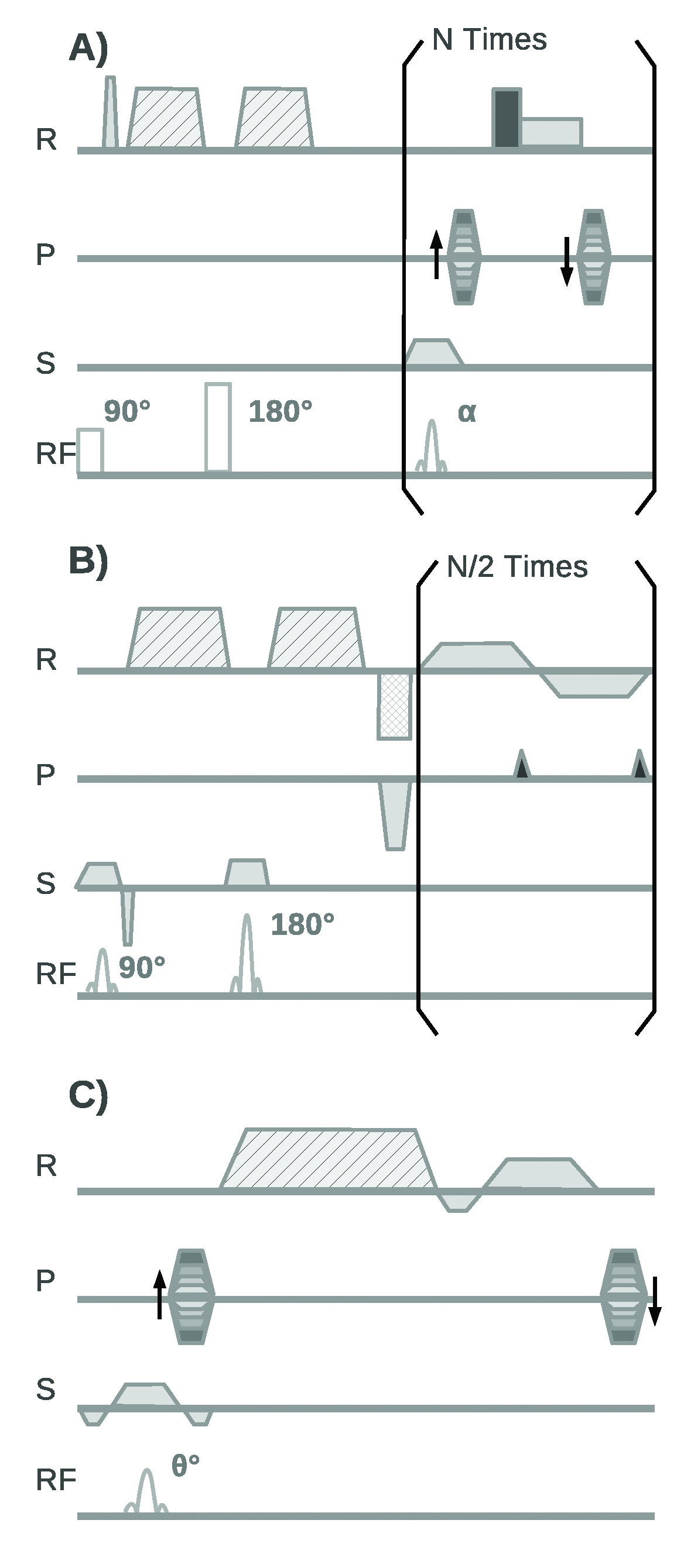
The diffusion sequences can in first place be classified as single shot (i.e. whole k-space is acquired after one excitation) and multiple shot sequences (i.e. k-space is acquired after several excitations). The advantages of single shot sequences are their fast acquisition and their robustness against macroscopic motion. However, single shot sequences have important disadvantages: They have characteristic long echo times (~80 ms), which limits the resolution that can be achieved, and they are susceptible to off-resonance. The two most popular single-shot diffusion sequences are the diffusion-weighted turbo spin echo (DW-TSE) and the diffusion-weighted echo planar imaging (DW-EPI) sequences. Both sequences have a diffusion-weighted spin echo preparation followed by a train of spin echo readouts (DW-TSE) or a train of gradient echo readouts (DW-EPI) to acquire the complete k-space (Fig. 2AB). The most broadly used sequences are the displaced ultra-fast low angle RARE sequence (displaced U-FLARE6, Fig. 2A) and the phase-insensitive RARE7 pulse sequence. The gradient echo readouts of DW-EPI have the advantage of a very efficient sampling of the excited magnetization, since the gradient echoes can be acquired one just after the other (Fig. 2B).8
Multiple shot sequences have much shorter echo times and therefore better signal-to-noise ratios (SNR) and allow for submillimeter image resolution. However, multiple shot sequences have long acquisition times and are very sensitive to macroscopic motion. If the subject moves while the diffusion sensitizing gradients are applied, all the spins in the knee will acquire an extra phase due to this macroscopic motion. Since the motion differs from one excitation to the next the phases in each line in k-space are different. This extra phase does not lead to additional signal decay, since all the spins in the voxel add the same extra phase, but effectively act as an incorrect phase encoding. Thus, if the phase differences are not corrected the final magnitude image usually presents a characteristic ghosting with multiple replicas of the image.9
Spin echo (SE) sequences have attractive advantages for diffusion imaging of MSK tissue (Fig. 3AB). The sensitivity of SE sequences to coherent macroscopic motions can be reduced either by modifying the image acquisition or by correcting the data after the MRI measurement. Example of strategies of the first is the line scan acqiuosotion in which the images is acquired line by line.10 Strategies to correct for coherent macroscopic motions after the image acquisition mostly use the navigator echo technique, which was independently proposed by Ordidge et al.11 and Anderson and Gore12 in 1994 (Fig. 3B). By the subtraction of these phases coherent motion artifacts can be to a great extent suppressed. Due to the complex motion that can occur in the knee 2D (or even 3D) navigators provide better motion correction.13
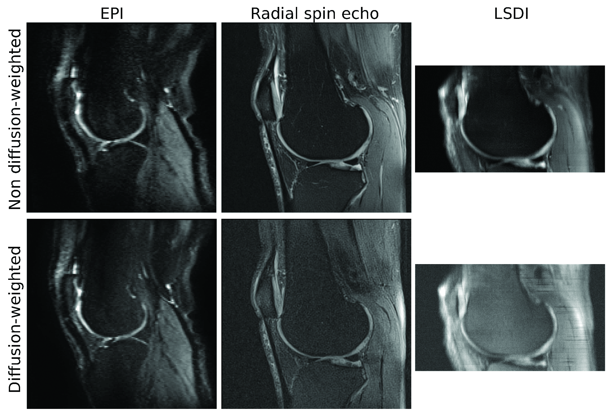
Figure 5 shows an example of different imaging sequences applied to diffusion-weighted imaging of articular cartilage.
Protocol optimization for DWI
Protocol optimization has to be carefully performed to balance the maximum diffusion-weighting used, the image resolution and the scanning time, so that SNR in the diffusion-weighted images is enough (SNR>5–10) to perform accurate estimations of the diffusion parameters.14
In this Section, we present some general recommendations for protocol optimization. These recommendations apply to almost any pulse sequence (SSFP and DESS sequences require other considerations) and are based on our experience. More detailed explanations about protocol optimization the reader should refer to the literature.14
We aim to optimize the SNR of a given tissue in the diffusion-weighted images, which is the limiting factor for the quality of the measured diffusion parameters. The rule of thumb is that the SNR in the diffusion-weighted images has to be at least 5. The SNR can be measured with different methods.15
While there is many ways on optimizing the protocol we like to start by optimizing the echo time and your maximum diffusion weighting. As a rule of thumb the optimal diffusion weighting is 1/D. For a diffusion weighting for a tissue with D=1.0–1.5×10⁻³ mm2/s, the optimal b-values are between 660 and 1000 s/mm2. Sometimes the optimal b-value is difficult to achieve due to the low signal and a lower b-value needs to be used. Once we choose a b-value, we select δ to be as short as possible by setting the gradients to the highest strength allowed. This will maximize your diffusion time and minimum TE. As an example, with a maximum gradient of 35 mT/m, which is available in most clinical scanners, the minimum echo time for a b-value of 660 s/mm2 is 50 ms, which means a remaining signal of , i.e. only 10% of the signal remains (assuming T2=40 ms and D=1.5×10⁻³ mm2/s).
Next we have to select a target resolution, which determines the matrix size of the image. For example, if we plan to measure the knee with a field of view in the phase direction of 154 mm with a 0.6 mm resolution we will need a 154/0.6=256 matrix. Depending on the type of sequence the matrix size will affect our TE, as is the case of EPI sequences. If TE goes more than twice the T2 of the tissue you will have too low signal. In sequences with SE-based preparation of the magnetization the repetition time should be ideally set to at least five times the T1 relaxation time to allow for full relaxation of the magnetization after each excitation. However, for multi-shot sequences the use of this optimal repetition time can result in prohibitive large acquisition times, so shorter repetition times of 1–2 s have to be considered. The loss in SNR for a given TR as compared with full recovery is , with T1 of 1 s (if we consider TR=1 s the signal loss is
, i.e. 37%).
For multi-shot sequence the trade-off between diffusion-weighting and echo time is even worse. For a DW-EPI using partial Fourier 5/8 and parallel imaging acceleration factor the shortest echo times available for a b-value of 400 s/mm2 are of the order of 80 ms (matrix 192×256), which means that only 6% of the signal is available at the echo time. The shorter acquisition times of single shot sequences allow multiple repetitions to compensate for their poor SNR.
The last remaining question is the number of directions that need to be acquired. The minimum number of direction included should in no case be less than three orthogonal directions if only the mean diffusivity is being measured. To measure DTI you will need to measure the diffusion along six or more different directions, in order to have a system of equations to estimate the components of the diffusion tensor. There have been extensive studies to analyze the optimal directions to perform DTI.14 A common metric to measure the performance of a direction encoding scheme is the condition number, which is per definition greater than 1 and the lower the better.18 Minimization of the condition number with six diffusion direction resulted in the “downhill simplex scheme” (DMS6) gradient (condition number=1.32).18 However, the DMS6 gradient schema may underperform depending on the orientation of the diffusion tensor with respect to the measured directions. Therefore, it is usually used the ichosaedral arrangement of directions, which perform equal independently of the orientation of the diffusion tensor.14
Depending on the acquisition time available it can be possible to include intermediary b-values or increase the number of averages to improve the SNR of the highest b-value images. The optimal strategy depend on how many diffusion weighted-images you can acquire. As an orientation, for a small number of images the precision of the diffusion parameters would improve more by averaging as by increasing the number of diffusion-weightings.16,17
Acknowledgements
No acknowledgement found.References
1. Novikov DS, Fieremans E, Jensen JH, Helpern JA. Random walk with barriers. Nature physics. 2011;7(6):508-514.
2. Novikov DS, Kiselev VG. Effective medium theory of a diffusion-weighted signal. NMR Biomed. 2010;23(7):682-697.
3. Mattiello J BP, Le Bihan D. The b matrix in diffusion tensor echo-planar imaging. Magn Reson Med. 1997;Feb;37(2):292-300.
4. Raya J, Dietrich O, Horng A, Weber J, Reiser M, Glaser C. T2 measurement in articular cartilage: impact of the fitting method on accuracy and precision at low SNR. Magnetic resonance in medicine : official journal of the Society of Magnetic Resonance in Medicine / Society of Magnetic Resonance in Medicine. 2010;63(1):181-193.
5. Basser PJ, Ozarslan E. Anisotropic diffusion: From the aparent diffusion coefficient to the apparent diffusion tensor. In: Jones DK, ed. Diffusion MRI: Theory, methods and applications. New York: Oxford University Press.
6. Norris DG. Ultrafast low-angle RARE: U-FLARE. Magnetic resonance in medicine : official journal of the Society of Magnetic Resonance in Medicine / Society of Magnetic Resonance in Medicine. 1991;17(2):539-542.
7. Alsop DC. Phase insensitive preparation of single-shot RARE: application to diffusion imaging in humans. Magnetic resonance in medicine : official journal of the Society of Magnetic Resonance in Medicine / Society of Magnetic Resonance in Medicine. 1997;38(4):527-538.
8. Skare ST, Bammer R. EPI-based pulse sequence for diffusion tensor MRI. In: Jones DK, ed. Diffusion MRI:Theory, methods and applications. New York: Oxford University Press; 2011:182-202.
9. Jones DK. Twenty-five pitfalls in the analysis of diffusion MRI data. NMR Biomed. 2010;23(7):803-820.
10. Gudbjartsson H, Maier SE, Mulkern RV, Morocz IA, Patz S, Jolesz FA. Line scan diffusion imaging. Magnetic resonance in medicine : official journal of the Society of Magnetic Resonance in Medicine / Society of Magnetic Resonance in Medicine. 1996;36(4):509-519.
11. Ordidge RJ, Helpern JA, Qing ZX, Knight RA, Nagesh V. Correction of motional artifacts in diffusion-weighted MR images using navigator echoes. Magn Reson Imaging. 1994;12(3):455-446.
12. Anderson AW, Gore JC. Analysis and correction of motion artifacts in diffusion weighted imaging. Magn Reson Med. 1994;32(3):379-387.
13. Miller KL, Pauly JM. Nonlinear phase correction for navigated diffusion imaging. Magn Reson Med. 2003;50(343-353).
14. Jones DK. Optimal approaches for MR acquisition In: Jones DK, ed. Diffusion MRI: Theory, methods and applications. New York: Oxford University Press; 2011:250-271.
15. Dietrich O, Raya JG, Reeder SB, Reiser MF, Schoenberg SO. Measurement of signal-to-noise ratios in MR images: influence of multichannel coils, parallel imaging, and reconstruction filters. Journal of magnetic resonance imaging : JMRI. 2007;26(2):375-385.
16. Jones JA, Hodgkinson P, Barker AL, Hore PJ. Optimal sampling strategies for the measurement of spin-spin relaxation times. J Magn Reson. 1996;113B:25-34.
17. Shrager RI, Weiss GH, Spencer RGS. Optimal sampling strategies for T2 measurements: monoexponential and biexponential systems. NMR Biomed. 1998;11:297-305.
18. Skare S, Hedehus M, Moseley ME, Li TQ. Condition number as a measure of noise performance of diffusion tensor data acquisition schemes with MRI. J Magn Reson. 2000;147:340-352.
Figures
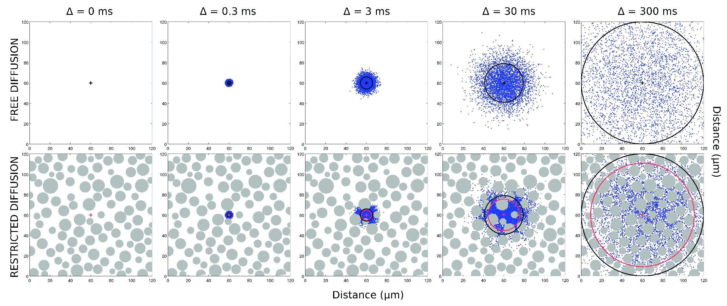
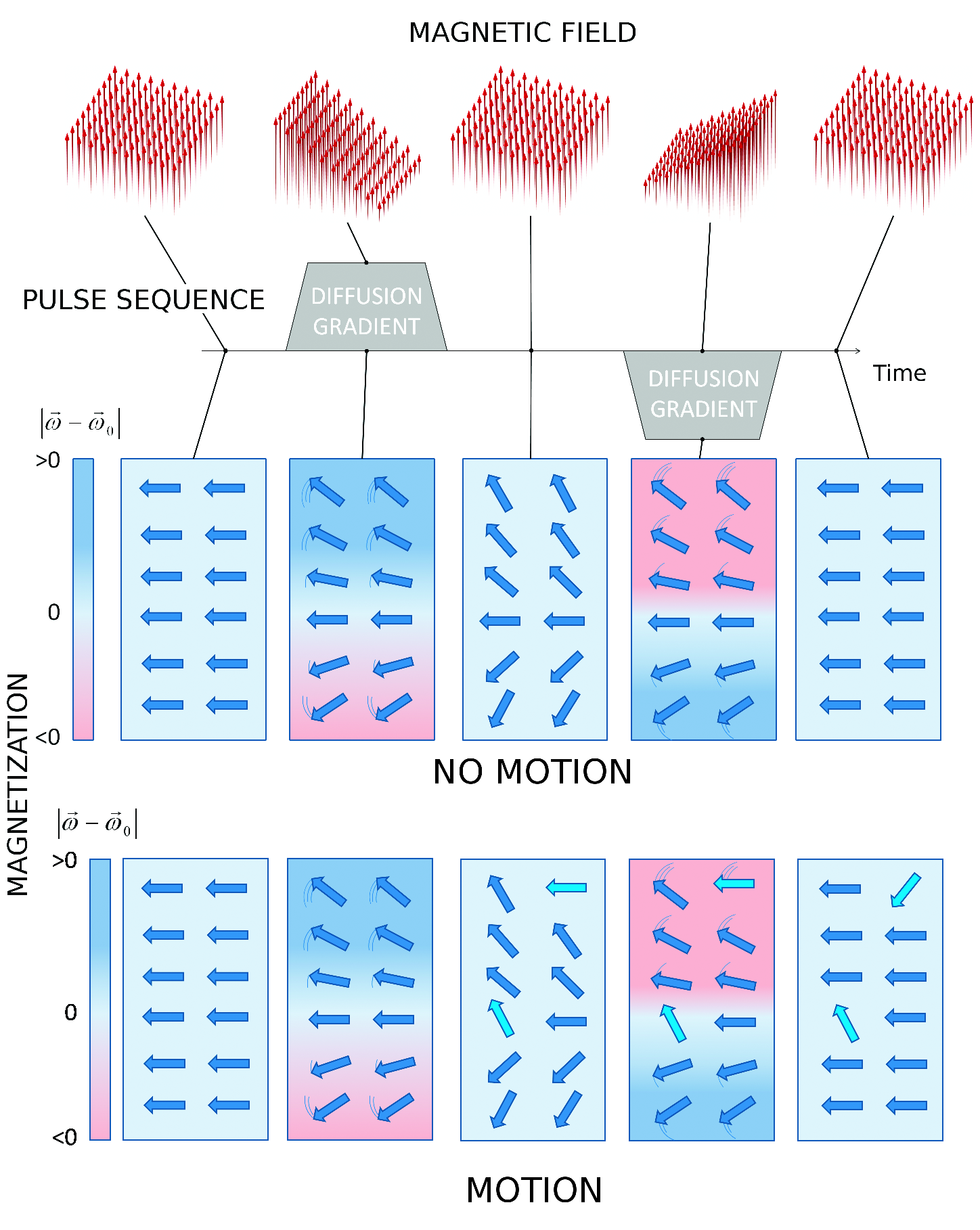
Illustration on how the diffusion sensitizing gradients (gray solid areas) act in the magnetization. The top row represents the magnetic field at different times and the no motion row shows the orientation of the transversal magnetization after a 90 degree excitation as seen by an observer who rotates with the Larmor frequency (![]() . At the beginning only the uniform component of the magnetic field is present. In the rotating frame the magnetization appears frozen. Once the magnetic gradient is applied the strength of the magnetic field changes linearly in space. Therefore the magnetization experiences a different frequency depending on their position and begins to dephase. The background color shows the precession frequency. Light blue indicate zero frequency (
. At the beginning only the uniform component of the magnetic field is present. In the rotating frame the magnetization appears frozen. Once the magnetic gradient is applied the strength of the magnetic field changes linearly in space. Therefore the magnetization experiences a different frequency depending on their position and begins to dephase. The background color shows the precession frequency. Light blue indicate zero frequency (![]() , darker blue indicated increased frequency (
, darker blue indicated increased frequency (![]() , and darker red decreasing frequency (
, and darker red decreasing frequency (![]() . The thin lines indicate direction of the rotation. Once the gradient is turned off the magnetization is frozen but magnetization remains dephased. With the second gradient the magnetization experience the opposite frequency as with the first gradient. After the gradients have been turned off the magnetization is completely rephased. The motion row represents the magnetization at the same points as in no motion row. However, during the diffusion time the magnetization change its position (light blue arrows). After the second gradient all the magnetization which did not move is refocused (dark blue arrows).
. The thin lines indicate direction of the rotation. Once the gradient is turned off the magnetization is frozen but magnetization remains dephased. With the second gradient the magnetization experience the opposite frequency as with the first gradient. After the gradients have been turned off the magnetization is completely rephased. The motion row represents the magnetization at the same points as in no motion row. However, during the diffusion time the magnetization change its position (light blue arrows). After the second gradient all the magnetization which did not move is refocused (dark blue arrows).