Sparsity & Compressed Sensing
1Radiology, University of Wisconsin, Madison, WI, United States
Synopsis
Incomplete data sampling is an attractive approach to accelerate MRI but it requires prior knowledge-driven image reconstruction. Sparsity is a powerful concept that allows linking many different types of prior knowledge to the mathematical apparatus adopted in MR image reconstruction. Compressed sensing theory establishes conditions for optimal use of sparse representations for high quality MR image reconstruction from undersampled data. In this talk, we will cover the aforementioned concepts of advanced image reconstruction and demonstrate real examples of accelerated structural and dynamic MRI. We will also discuss both theoretical requirements of compressed sensing and essential aspects of its practical implementation.
Highlights
- Incomplete data sampling is an attractive approach to accelerate MRI but requires prior knowledge-driven MR image reconstruction.
- Sparsity is a powerful concept that allows linking many different types of prior knowledge to the mathematical apparatus adopted in MR image reconstruction.
- Compressed sensing theory establishes criteria relating image sparsity and admissible undersampling strategies, and allows establishing feasible image reconstruction algorithms from incomplete data.
Target Audience
Physicists and engineers who wish to acquire an understanding of advanced MR image reconstruction based on prior knowledge-driven techniques.Outcome/Objectives
- Develop a basic understanding of how image acquisition can be accelerated by undersampling strategies and how employing prior knowledge of object sparsity can be utilized to restore missing data and obtain MR images of diagnostic quality
- Develop a basic understanding of essential results of the compressed sensing theory
Introduction
In MRI, a digital image needs to be estimated from a discrete set of measurements, each sample representing an integral of the image modulated by encoding function composed of magnetic field gradient and coil sensitivity contributions. In the matrix form, the set of measurements (i.e., signal vector) is modeled by
\begin{equation}s=Ef+\epsilon,\qquad\qquad\qquad[1]\end{equation}
where $$$f$$$ is the column vector of length $$$M$$$ corresponding to the image to be estimated, $$$E$$$ is the encoding matrix, and $$$\epsilon$$$ is measurement noise. Assuming that the problem is overdetermined (i.e., the number of linearly independent rows, or row rank of $$$E$$$, is higher than the number of unknowns $$$M$$$) and assuming independent noise, an SNR-optimized image reconstruction can be accomplished in the least squares sense:
$$f=\arg\min_f\|Ef-s\|_2^2,\qquad\qquad[2]$$
where $$$\|\cdot\|_2$$$ is $$$l_2$$$ norm defined as
$$\|x\|_p=\left(\sum_k|x|^p\right)^{1/p}\qquad\qquad[3]$$
with $$$p=2$$$.
Achieving higher spatial and/or temporal resolutions in MRI often necessitates incomplete data sampling, which, in turn, leads to poorly conditioned and, in the limiting case, underdetermined system of equations in Eq. [1] (row rank ($$$E$$$) < $$$M$$$), which generally have an infinite number of possible solutions. A common approach to isolate a feasible solution is to incorporate additional prior information about the problem at hand to restore images of diagnostic quality from the undersampled data (1-3). This, in turn, requires modifications to the least square estimation problem in Eq. [2] and leads to specialized reconstruction algorithms. In this presentation, we will describe a subset of such algorithms based on principles of sparse optimization.
Sparsity in MRI
Sparsity is a powerful concept that allows linking many different types of prior knowledge to the mathematical apparatus adopted in MR image reconstruction. A strict definition requires a sparse image object to have few non-zero entries. Figure 1a shows an example of MR image, which can be practically described as naturally sparse (to the level of residual signal in the background). More often, MR images are not naturally sparse, and a mathematical operation $$$\Phi$$$ may be needed to transform them into a space in which they can be considered sparse. An example of such a transformation is shown in Figs. 1b,c. The sparsity of a solution or its transformation can be quantified by suitable mathematical norms and incorporated into MR image reconstruction to isolate sparse solutions to the underdetermined problem as described next.Mathematical Measures of Sparsity and Their Use in Image Reconstruction
Ideally, the sparsity of an image is measured by its $$$l_0$$$ norm that counts the number of non-zero pixels. (Note that despite the name $$$l_0$$$ norm is technically not a norm as it does not satisfy all the necessary axioms). If we know in advance that the underlying image or its transformation is expected to be sparse, then the problem of MR image estimation from undersampled data may be modified by combining data consistency (Eq. [2]) and sparsity information in the form of additional regularization term as follows:
$$f=\arg\min_f\left(\|Ef-s\|_2^2+\lambda\|\Phi f\|_0\right).\qquad\qquad[4]$$
The ability of $$$l_0$$$ norm regularization to isolate a sparse solution is illustrated in Fig. 2a. However, the practical implementation of $$$l_0$$$-based problems is complicated due to combinatorial complexity of suitable optimization algorithms. The use of alternative norms may not always lead to sparse solutions. For example, Figure 2b demonstrates that using a more traditional $$$l_2$$$ norm results in a non-sparse solution. However, as can be seen from Figure 2c, optimization based on $$$l_1$$$ norm also produces a sparse solution and, importantly, is computationally tractable. Establishing a set of conditions warranting equivalency of $$$l_0$$$ and $$$l_1$$$ norm optimization was one of the milestones of the compressed sensing theory described below.
Compressed Sensing Theory
Recently, a novel mathematical theory named compressed sensing (CS) has been developed (4) that states that sparse images can be accurately reconstructed from undersampled datasets, provided the encoding matrix $$$E$$$ satisfies certain conditions. The first of these conditions, called Restricted Isometry Principle (RIP), requires that most of the energy of a sparse signal should be preserved with measurements performed via the encoding matrix $$$E$$$. As such, RIP guarantees that different sparse images produce different sets of measurements and thus can be differentiated in the reconstruction process. In practice, RIP can be achieved by incoherence of the sampling pattern and, in MRI applications, can be well approximated by randomized or non-Cartesian acquisitions. The second theoretical condition of CS relates the sparsity level of the signal with admissible acceleration factors. Under these conditions, CS theory proves that the $$$l_0$$$ and $$$l_1$$$ minimization problems result in equivalent solutions, i.e. we can solve the following problem instead of the one in Eq. [4]:
$$f=\arg\min_f\left(\|Ef-s\|_2^2+\lambda\|\Phi f\|_1\right)\qquad\qquad[5]$$
While historically a number of algorithms in the form of Eq. [5] were proposed earlier, including MRI algorithms (5-7), the compressed sensing theory was the first to formulate sufficient conditions on the number of samples and the encoding matrix to guarantee accurate sparse signal recovery, and later was applied in the context of MRI (8).
Conclusion
In this talk, we will cover the aforementioned aspects of advanced MR image reconstruction. We will additionally demonstrate real world examples of its application for accelerating structural and dynamic MRI. We will also discuss both theoretical requirements of compressed sensing and some aspects of its practical implementation.Acknowledgements
No acknowledgement found.References
1. Liang ZP, Lauterbur PC. An efficient method for dynamic magnetic resonance imaging. IEEE Trans Med Imag, 1994; 13: 677-686.
2. Tsao J, Boesiger P, Pruessmann KP. k-t BLAST and k-t SENSE: dynamic MRI with high frame rate exploiting spatiotemporal correlations, Magn Reson Med, 2003; 50: 1031-1042.
3. Samsonov AA, Kholmovski EG, Parker DL, Johnson CR. POCSENSE: POCS-based reconstruction for sensitivity encoded magnetic resonance imaging. Magn Reson Med, 2004; 52: 1397-1406.
4. Candès EJ, Romberg J. Sparsity and incoherence in compressive sampling. Inverse Problems, 2007; 23:969-985.
5. O. Portniaguine, C. Bonifasi, E. V. R. DiBella, and R. T.Whitaker RT. Inverse methods for reduced k-space acquisition. Proceedings of ISMRM, 2003; p.481.
6. Velikina JV. VAMPIRE: Variation Minimizing Parallel Imaging Reconstruction. Proceedings of ISMRM 2005; p. 2424.
7. Block KT, Uecker M, Frahm J. Undersampled radial MRI with multiple coils. Iterative image reconstruction using a total variation constraint. Magn Reson Med, 2007; 57(6):1086-1098.
8. Lustig M, Donoho D, Pauly JM. Sparse MRI: The application of compressed sensing for rapid MR imaging. Magn Reson Med, 2007; 58(6):1182-1195.
Figures
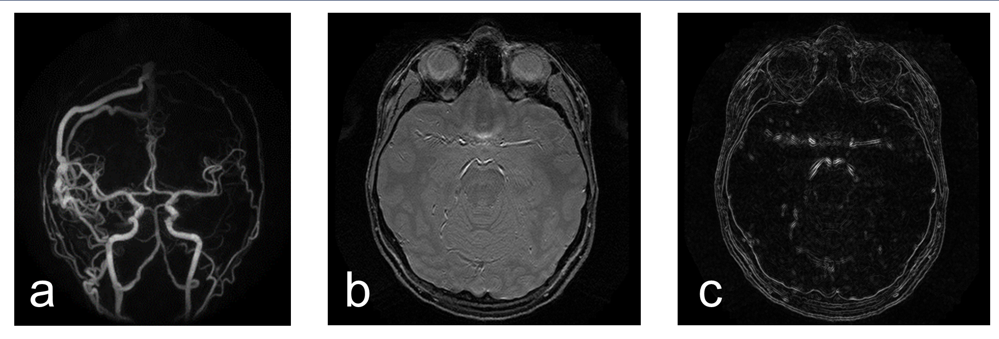
Figure 1. Examples of native and transform sparsity in MRI. (a) MR angiogram can be described as naturally sparse due to the large number of relatively low intensity pixels corresponding to air and suppressed brain tissue. No additional image transformation is needed in the case ($$$\Phi=\text{Identity}$$$). (b) Proton density-weighted MR image of the brain is not sparse. (c) An application of spatial derivative transformation ($$$\Phi=D$$$) to image in (b) efficiently sparsifies it.

Figure 2. Examples of recovery of a signal with two entries by minimizing its (a) $$$l_0$$$, (b) $$$l_2$$$, and (c) $$$l_1$$$ norm subject to data consistency condition (geometrically, a hyperplane in the signal space). Being non-convex, both $$$l_0$$$ and $$$l_1$$$ norms lead to a sparse solution with only one non-zero coordinate, while the use of convex $$$l_2$$$ norm results in a non-sparse solution with two non-zero coordinates.