Synopsis

Introduction

Background concepts

Hard pulse excitation

The simplest excitation pulse is a ‘hard’ pulse, which has constant magnitude and phase. Because MRI systems generate RF pulses using sample-and-hold DAC circuitry, all RF pulses can be accurately modeled as a series of short hard pulses of varying amplitude and phase. Magnetization rotates in a plane perpendicular to a hard pulse’s field vector. For example, if a hard pulse is applied along the x-axis, magnetization is rotated in the y-z plane. The flip angle excited by a hard pulse is simply its duration T, multiplied by its magnitude |B1| and the gyromagnetic ratio γ:

$$\theta = \gamma |B_1| T$$

While we will make use of the hard pulse as a theoretical tool for understanding more complex RF pulses, hard pulses are commonly used for excitation in 3D sequences, where the three spatial dimensions are resolved by the imaging readout.

Types of excitation operations

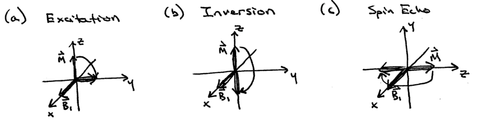
All of the pulses we will discuss are used to do one of three things. RF pulses are most commonly used to excite magnetization from the z axis into the x-y plane so that it will precess and produce a signal. This process is illustrated in Fig. 1a. There are also scenarios in which an ‘inversion’ is desired, as illustrated in Fig. 1b: here the goal is to rotate magnetization pointing along the positive z-axis by π radians, to the negative z-axis. Inversion pulses are used to prepare magnetization prior to an imaging readout, and they allow the user to modulate image contrast selectively for different chemical species based on their longitudinal relaxation time T1. The third excitation operation is a spin echo and is also a π rotation, whose effect is illustrated in Fig. 1c. Spin echo pulses are most commonly applied midway between an excitation and image readout, and are used to refocus magnetization that is dephased due to off-resonance, as they have the effect of conjugating the phase of magnetization lying in the transverse plane. This makes T2- weighted imaging with long echo times possible, since the spin echo pulse reverses phase dispersion that would otherwise result in signal loss.

Small-tip excitation and excitation k-space

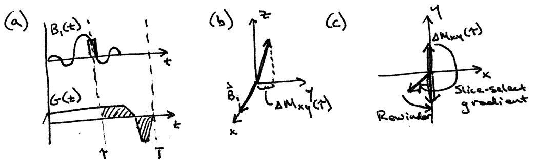
The small-tip-angle approximation [1], which we derive graphically here, is an extremely useful mathemat- ical and interpretational tool. Consider the shaped RF pulse B1(t) in Fig. 2a, played out concurrently with a gradient G(t). If the final flip angle pattern excited by this pulse is small (less than about 30◦), and if the intermediate flip angles reached during its playout are also small, then one can assume with reasonable accuracy that the longitudinal (Mz) component of the magnetization is unperturbed by the pulse. Then the pulse can be decomposed into a series of very short hard subpulses, each of which creates a small amount of transverse magnetization. Consider time point τ, indicated in Fig. 2a. As illustrated in Fig. 2b, the small rotation induced by the RF at this time point creates a small amount of transverse magnetization given by:

$$\Delta M_{xy}(\tau) = i \gamma M_0 B_1(\tau) \Delta t,$$

where ∆t is the duration of the hard subpulse. Because ∆Mxy (τ ) was not created until τ , it is unaffected by the gradient field prior to τ; it only sees the gradient field after τ, which is depicted as the shaded gradient area in Fig. 2a. Let's define the ‘excitation k-space trajectory’ k(τ) as the remaining gradient area (in units of cycles per cm):

$$k(\tau) = -\frac{\gamma}{2\pi} \int_{\tau}^T G(s)ds,$$

where T is the end of the gradient waveform. At time T, the magnetization created at time τ will have accrued phase due to the remaining gradients, so that at spatial position z the magnetization created at time τ and observed at time T will be given by:

$$i \gamma M_0 B_1(\tau) \Delta t e^{i2\pi k(\tau) z}.$$

Summing all the small magnetization components created during the RF pulse, we obtain the final magneti- zation pattern excited by the pulse (in the limit as ∆t approaches zero):

$$M_{xy}(z,T) = i \gamma M_0 \int_0^T B_1 (t) e^{i2\pi k(t) z} dt,$$

i.e., the final magnetization pattern is the Fourier transform of the RF pulse, evaluated along the excitation k-space trajectory!

Frequency-selective excitation

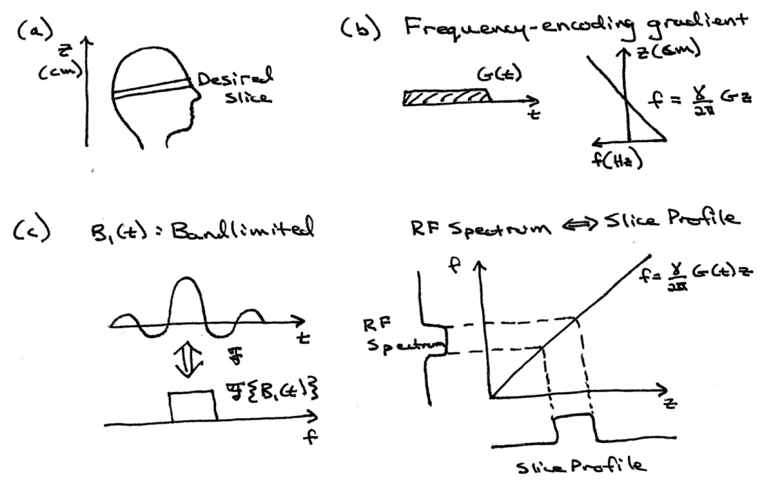
In most MR imaging scenarios, it is desirable to limit the volume over which we acquire signal, and we can use frequency-selective RF pulses to achieve this goal. Figure 3a shows an example scenario in which we want to limit the signal volume to a single slice in the head; gradients would then be used during readout to resolve the x and y dimensions. Therefore, we would like an RF pulse to selectively excite magnetization only within this slice. Note that the z profile of the desired slice is a rectangular function, with a uniform flip angle inside the slice and zero flip angle outside. To excite this slice only, we will use the z-gradient to create a one-to-one mapping of spatial location to resonant frequency. Figure 3b shows that a constant z gradient will create a linear resonant frequency variation in z. During the gradient pulse we will simultaneously play out a small-tip-angle bandlimited RF pulse, whose Fourier transform is (approximately, due to finite pulse duration) a rectangular function. As we showed in the previous section, the spatial magnetization pattern excited by this pulse is equal to its Fourier transform, so we have achieved our goal of selectively exciting only the desired slice.

Bloch equation non-linearity

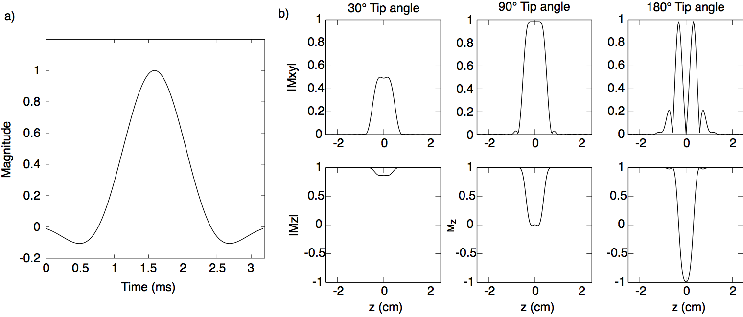
The small-tip-angle approximation yields a straightforward method for designing RF pulses: given the desired excitation pattern, one simply needs to define an excitation k-space trajectory that samples it sufficiently, and determine the RF pulse as the Fourier transform of the pattern along the trajectory. However, in reality the Bloch equation governing the response of magnetization to RF excitation is non-linear, so more sophisticated pulse design methods are necessary at tip angles larger than about 45◦. Figure 4 illustrates the effects of Bloch equation non-linearity on a slice-selective pulse designed using the small-tip-angle approximation (Fig. 4a). Figure 4b shows the transverse (Mxy) and longitudinal (Mz) magnetization profiles excited by this pulse, after it has been scaled to produce 30◦, 90◦, and 180◦ tip angles in the center of the slice. At 30◦ tip, the pattern contains no visible ripples outside the slice. At 90◦ tip, we start to see ripples outside the slice, and the ripple inside the slice has flattened out. The Mz profile also narrows at 90◦. At 180◦ tip (corresponding to an inversion), more out-of-slice ripples appear, and the transverse magnetization has decreased in the center of the slice, while the Mz profile has narrowed further and Mz = −1 in the slice center. This illustration demonstrates that specialized design techniques are necessary to obtain accurate large-tip-angle RF pulses.

RF pulse classes and their applications

One-dimensional slice-selective pulses

Most RF pulses used in practice are one-dimensional slice-selective pulses, which we have illustrated in the ‘Frequency-selective excitation’ section. These pulses are used for all three types of excitation operations. For small-tip-angle excitation, these pulses are commonly chosen to be Hamming-windowed sincs, where the windowing is used to control pulse truncation effects (i.e., Gibbs ringing) on the slice profile. Despite Bloch-equation nonlinearity at large-tip-angles, Hamming-windowed sincs are commonly used as spin echo pulses, where the undesirable sidelobes that arise in their excitation patterns at large-tip-angles are crushed away by large gradient pulses played before and after the pulse. For more accurate large-tip-angle excitation a pulse may be designed using advanced techniques such as the Shinnar-Le Roux algorithm [2], optimal control [3], and the inverse scattering transform [4]. The Shinnar-Le Roux algorithm is the most frequently employed method for directly designing large-tip-angle slice-selective pulses. Multiband slice-selective pulses for simultaneous multislice imaging are typically constructed by summing a set of identical slice-selective pulses, after modulating each pulse to its slice location.

Most one-dimensional slice-selective pulses are designed to leave a linear phase ramp across the excited slice, that can be easily refocused using a gradient blip. However, pulses that excite non-linear phase patterns (e.g., quadratic) can have significantly lower peak RF magnitude for a given slice profile [5]. Compared to a linear phase pulse, when employed in inversion or saturation operations (i.e., excitation operations in which the phase profile is inconsequential) non-linear phase pulses can be used to either excite sharper slice profiles at the same peak RF magnitude, or reduce RF magnitude for a fixed slice profile.

Adiabatic pulses

Adiabatic pulses [6] are a special class of pulse that are capable of exciting, inverting or refocusing spins uniformly across an object in the presence of strong RF field strength (|B1|) inhomogeneities. Such inhomo- geneities cause conventional pulses to excite undesirable spatially-nonuniform flip angle patterns, especially on high field MRI scanners. Adiabatic pulses operate under the adiabatic passage principle, which states that magnetization that is initially parallel to the effective magnetic field (comprised of the vector sum of the transverse B1 and longitudinal RF frequency modulation fields) will follow the direction of that field, so long as the effective field does not change its direction much during one rotational period of the magnetization around the effective field. Adiabatic pulses are useful in many imaging scenarios that demand uniform excitation.

The hyperbolic secant pulse [7] is commonly used for adiabatic inversion, to induce T1 weighting and to null fat signal via inversion recovery [8, 9]. To invert magnetization, the pulse's frequency modulation starts far off-resonance and the envelope starts small, so that the effective field points along the positive z axis, which is the initial direction of the magnetization. As time progresses, the RF envelope slowly increases, while the modulation approaches resonance, so that the effective field and the magnetization approach the transverse plane. As the envelope decreases again and the frequency modulation becomes off-resonant in the opposite direction, the effective field slowly moves to the -z axis, and the magnetization follows it. Above a certain RF magnitude threshold, and within a certain band of frequency offsets, the hyperbolic secant pulse is immune to RF field strength variations. Adiabatic pulses are not used for all RF excitation operations because of their long duration and/or high RF magnitude, and because they leave nonlinear phase profiles across a selected slice, but they can be used for refocusing in pairs, since the nonlinear phase produced by the first refocusing pulse will be canceled by the second.

Two-dimensional spatially-selective pulses

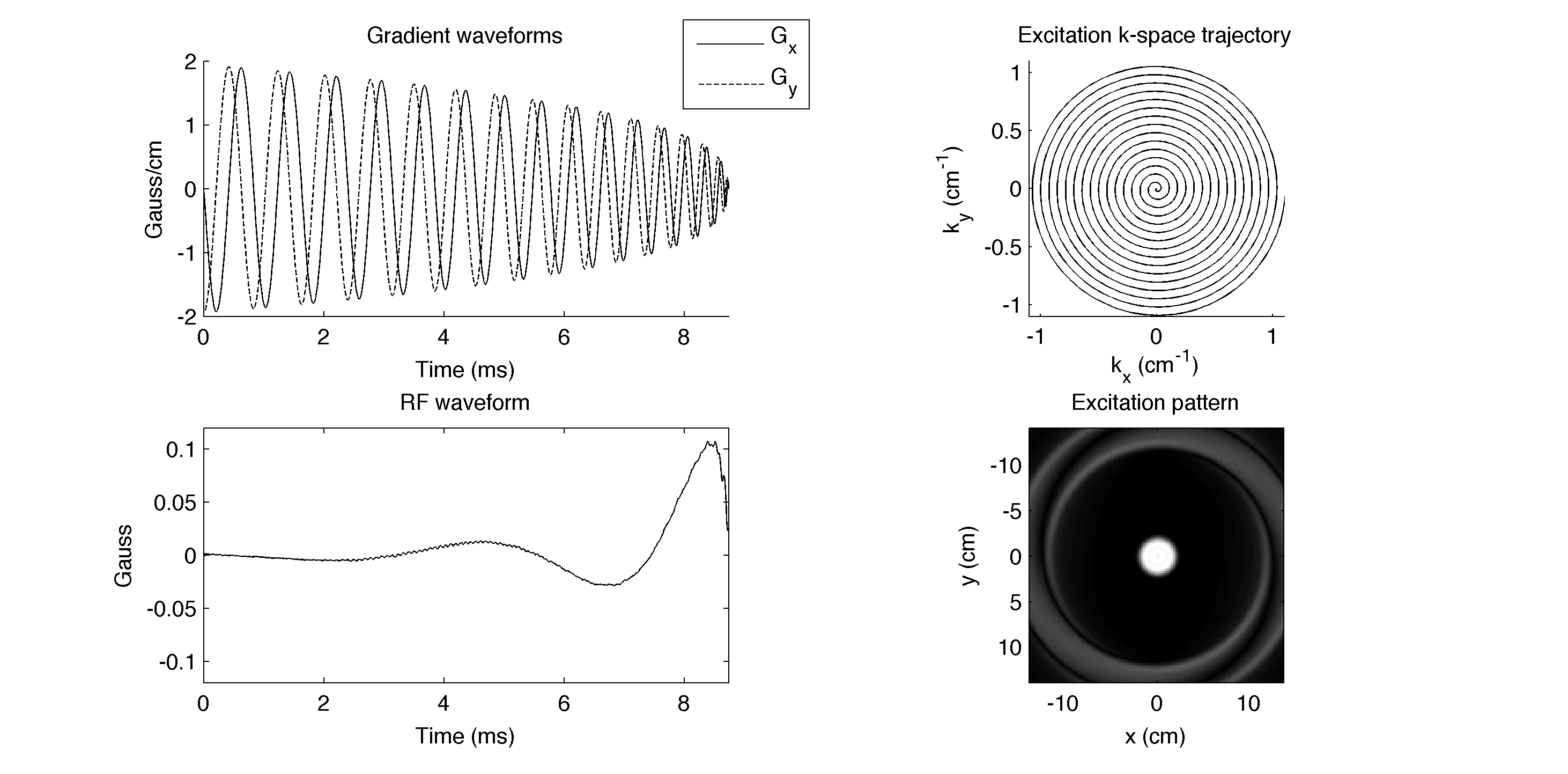
Two-dimensional spatially-selective RF pulses are used to limit the imaged volume in two dimensions, or to excite navigator signals. In the small-tip-angle regime, these pulses are commonly designed using Fourier analysis [1, 10], and under certain conditions on the trajectory and excitation pattern, they can also be scaled to excite large-tip-angles without incurring significant pattern distortion due to Bloch equation non-linearity [11]. Pulses that do not meet these conditions are typically designed using numerical optimization tech- niques [3, 12], though large-tip-angle echo-planar pulses can be designed using a Shinnar-Le Roux-based method applied sequentially in the slow (or blipped) and fast dimensions of the trajectory [13]. The most common types of two-dimensional spatially-selective excitation pulses are spiral and echo-planar pulses; a spiral pulse is illustrated in Fig. 5.

Spectral-spatial pulses

Whereas one-dimensional spatially-selective pulses are typically short enough to excite the same flip angle pattern across a wide range of resonant frequencies, spectral-spatial pulses [14] are used to selectively excite magnetization in both spectral and spatial dimensions. They are only selective in one spatial dimension, and are formed as a train of slice-selective subpulses that are weighted by a spectrally-selective envelope. The gradient waveforms oscillate to navigate back and forth in the slice-selective dimension, while the spectral k-space dimension evolves at a constant rate. Spectral-spatial are most commonly used to separate fat and water, e.g., to excite only water while leaving fat unperturbed, or to selectively suppress only the water or fat signals. They have also found applications in spectroscopic imaging, to suppress water or excite variable flip angles across a chemical shift spectrum [15, 16]. These pulses are usually designed using Fourier analysis, and can be designed separably, by weighting a train of slice-selective pulses with a spectrally-selective envelope [14], or using optimization techniques [17, 18].

Parallel transmission

Parallel transmission can address several problems in high field MRI, by providing an additional spatial encoding mechanism (the multiple channels and coils of a parallel transmit system) that enhances one’s ability to tailor excitation pulses to specific patients and anatomy [19, 20]. Small-tip-angle multidimensional designs are simplified by linearity of the spatial excitation pattern in the RF pulses, which enables pulse design by matrix inversion or iterative methods [21]. Pulse design requires the co-design of an excitation k-space trajectory, which is based on considerations of pulse duration, excitation FOV, and the required sharpness of the excitation pattern. The B1+ patterns of each coil must be included in the forward excitation model, and are generally measured in each subject prior to pulse design. Target excitation patterns and excitation error weighting can be constructed to approximately achieve target flip angle ripple levels [22]. SAR evaluation is straightforward for a given set of pulses, but ideally both local and global SAR are constrained during pulse design. The number of local SAR constraints can be reduced several orders of magnitude using virtual observation points [23]. Large-tip-angle parallel transmit pulse design is generally based on extensions of optimal control to the multi-channel case [24–27].

Acknowledgements

References

[1] J M Pauly, D G Nishimura, and A Macovski. A k-space analysis of small-tip-angle excitation. J Magn Reson, 81:43–56, 1989.

[2] J M Pauly, P Le Roux, D G Nishimura, and A Macovski. Parameter relations for the Shinnar-Le Roux selective excitation pulse design algorithm. IEEE Trans Med Imaging, 10:53–65, 1991.

[3] S Conolly, D Nishimura, and A Macovski. Optimal control solutions to the magnetic resonance selec- tive excitation problem. IEEE Trans Med Imaging, 5:106–115, 1986.

[4] M H Buonocore. RF pulse design using the inverse scattering transform. Magn Reson Med, 29(4):470– 477, Apr 1993.

[5] R F Schulte, J Tsao, P Boesiger, and K P Pruessmann. Equi-ripple design of quadratic-phase RF pulses. J Magn Reson, 166(1):111–122, 2004.

[6] M Garwood and L DelaBarre. The return of the frequency sweep: designing adiabatic pulses for contemporary NMR. J Magn Reson, 153(2):155–177, Dec 2001.

[7] M S Silver, R I Joseph, and D I Hoult. Highly selective π/2 and π pulse generation. J Magn Reson, 59:347–351, 1984.

[8] G M Bydder and I R Young. MR imaging: Clinical use of the inversion recovery sequence. J Comput Assist Tomogr, 9:659–675, 1985.

[9] G M Bydder, R E Steiner, and L H Blumgart. MR imaging of the liver using short TI inversion recovery. J Comput Assist Tomogr, 9:1084–1089, 1985.

[10] C Y Yip, J A Fessler, and D C Noll. Iterative RF pulse design for multidimensional, small-tip-angle selective excitation. Magn Reson Med, 54(4):908–917, Oct 2005.

[11] J M Pauly, D G Nishimura, and A Macovski. A linear class of large-tip-angle selective excitation pulses. J Magn Reson, 82(3):571–587, 1989.

[12] C Hardy, P Bottomley, M O’Donnell, and P Roemer. Optimization of two-dimensional spatially selec- tive NMR pulses by simulated annealing. J Magn Reson, 77:233–250, 1988.

[13] J M Pauly, D Spielman, and A Macovski. Echo-planar spin-echo and inversion pulses. Magn Reson Med, 29(6):776–782, Jun 1993.

[14] C H Meyer, J M Pauly, A Macovski, and D G Nishimura. Simultaneous spatial and spectral selective excitation. Magn Reson Med, 15(2):287–304, Aug 1990.

[15] A A Schricker, J M Pauly, J Kurhanewicz, M G Swanson, and D B Vigneron. Dual band spectral-spatial RF pulses for prostate MR spectroscopic imaging. Magn Reson Med, 46(6):1079–1087, 2001.

[16] P E Z Larson, A B Kerr, A P Chen, M S Lustig, M L Zierhut, S Hu, C H Cunningham, J M Pauly, J Kurhanewicz, and D B Vigneron. Multiband excitation pulses for hyperpolarized 13C dynamic chemical-shift imaging. J Magn Reson, 2008.

[17] C Y Yip, D Yoon, V T Olafsson, S Lee, W A Grissom, J A Fessler, and D C Noll. Spectral-spatial pulse design for through-plane phase precompensatory slice selection in T2∗-weighted functional MRI. Magn Reson Med, 61(5):1137–1147, 2009.

[18] W A Grissom, A B Kerr, A B Holbrook, J M Pauly, and K Butts-Pauly. Maximum linear-phase spectral-spatial radiofrequency pulses for fat-suppressed proton resonance frequency-shift MR ther- mometry. Magn Reson Med, 62(5):1242–1250, 2009.

[19] U Katscher, P Bo ¨rnert, C Leussler, and J S van den Brink. Transmit SENSE. Magn Reson Med, 49(1):144–150, Jan 2003.

[20] Y Zhu. Parallel excitation with an array of transmit coils. Magn Reson Med, 51(4):775–784, Apr 2004.

[21] W A Grissom, C Y Yip, Z Zhang, V A Stenger, J A Fessler, and D C Noll. Spatial domain method for the design of RF pulses in multicoil parallel excitation. Magn Reson Med, 56(3):620–9, Sep 2006.

[22] W A Grissom, A B Kerr, P Stang, G C Scott, and J M Pauly. Minimum envelope roughness pulse design for reduced amplifier distortion in parallel excitation. Magn Reson Med, 64(5):1433–1440, 2010.

[23] G Eichfelder and M Gebhardt. Local specific absorption rate control for parallel transmission by virtual observation points. Magn Reson Med, 66:1468–76, 2011.

[24] W A Grissom, C Y Yip, S M Wright, J A Fessler, and D C Noll. Additive angle method for fast large-tip-angle RF pulse design in parallel excitation. Magn Reson Med, 59(4):779–787, 2008.

[25] W A Grissom, D Xu, A B Kerr, J A Fessler, and D C Noll. Fast large-tip-angle multidimensional and parallel RF pulse design in MRI. IEEE Trans Med Imaging, 28(10):1548–1559, Oct. 2009.

[26] D Xu, K F King, Y Zhu, G C McKinnon, and Z-P Liang. Designing multichannel, multidimensional, arbitrary flip angle RF pulses using an optimal control approach. Magn Reson Med, 59(3):547–560, 2008.

[27] Z Cao, M J Donahue, J Ma, and W A Grissom. Joint design of large-tip-angle parallel RF pulses and blipped gradient trajectories. Magn Reson Med, 75(3):1198–1208, 2016.