Basics of Transmission Lines & Power Transfer
1Advanced MRI Section of the Laboratory of Functional and Molecular Imaging, National Institute of Neurological Disorders and Strokes, National Institutes of Health
Synopsis
Fundamentals of transmission lines and power transfer are presented to help in the understanding, design, implementation and performance evaluation of MRI hardware.
Target Audience
Those interested in understanding some of the concepts behind common radiofrequency (RF) interconnections in the MRI hardware setup.Objective
This talk will cover the following topics:
- Distributed-circuit analysis and wave equation of terminated transmission line (TL)
- Type of TLs commonly used in MRI
- Scattering parameters and the Schmitt chart, TL impedance and reflection coefficient
- TL applications in MRI: Impedance matching, balanced to unbalanced connection, cable traps, power splitting and monitoring, phase shifting, preamplifier decoupling, and coil design.
- TL practical considerations and TL lumped element equivalents
- Non-conventional power transfer in MRI
Introduction
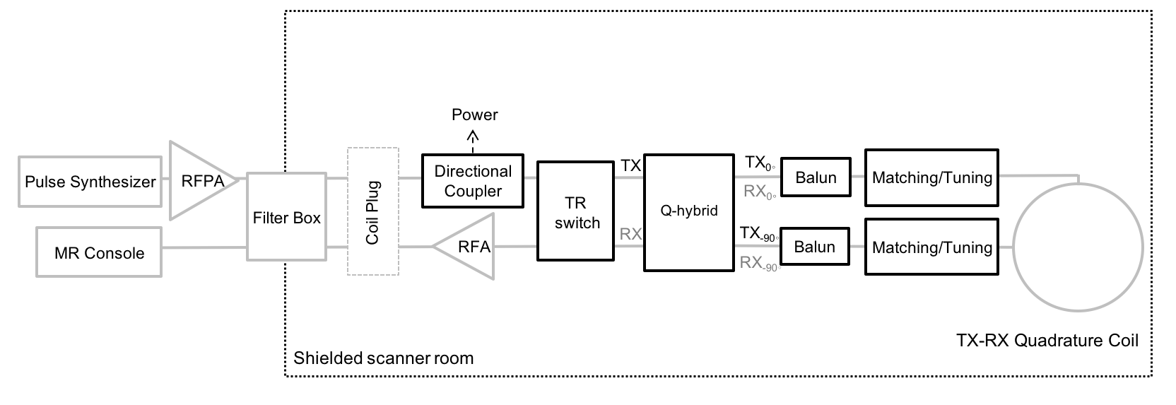
During both the excitation and acquisition phases of the MRI experiment, RF signals need to travel efficiently between the scanner system and the MR coils. In the conventional MRI setup, the coil and the scanner are interconnected through coaxial cables, which is a type of shielded transmission line that allows power to be transferred from one point to the other, ideally without radiation losses. As an example, Figure 1 shows a quadrature volume excitation and detection setup. Power is transferred from the power amplifier (RFPA) located in the equipment room to the coil plug located in the scanner bore through a long coaxial connection. There are multiple RF interconnections between the system and the coil, built from transmission line segments or their lumped element equivalent implementation (LC network). The impedance of interconnecting devices and coil (coupled to a nominal load) are matched to the characteristic impedance of the coaxial cable (MRI standard 50 Ω) for maximum power transfer. In the setup shown in Figure 1,
an
RF switch (Transmit/Receive switch) is used to add isolation between the low-power receiver’s
electronics, mainly the receive (RX) RF amplifier (RFA or preamplifier), and the
high-power RF transmit (TX) signal.
The single transmit signal is divided into two 90-degrees out-of-phase signals through a quadrature-hybrid (Q-hybrid). These quadrature signals drive two 90-degrees out-of-phase feed ports of the quadrature coil to generate a circularly polarized field. During signal reception, the hybrid will combine the two quadrature detected signals to be transmitted to the RFA. An RF coupler can be inserted in the transmit line to measure total power delivered to the coil under a specific load condition. A balun (balanced to unbalanced) or cable trap is used in coaxial connections to suppress RF currents on the cable’s shield, which can reduce system performance and compromise safety.
TL Basics
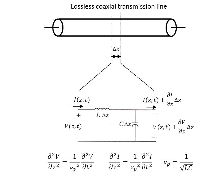
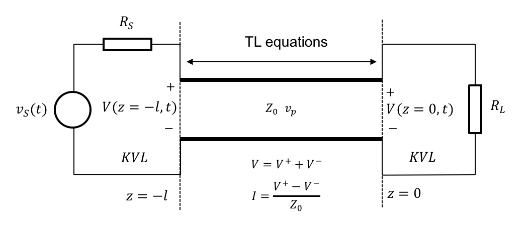
A TL transports electromagnetic energy from a source to a load in the form of a transverse electromagnetic (TEM) wave. A TEM wave has null electrical and magnetic field components in the direction of propagation (z). Some common TLs with their magnetic ($$$\overrightarrow{H}$$$) and electrical field ($$$\overrightarrow{E}$$$) vectors highlighted are shown in Figure 2. A differential segment of a lossless transmission line can be modeled as a series inductance connected to a shunt capacitance as shown in Figure 3. L and C are the distributed (in units per length) inductance and capacitance respectively. The TL (wave) equations (shown in the figure) can be formulated from this differential length model applying Kirchhoff’s current and voltage laws (KCL and KVL). A lossless TL can transport electromagnetic energy from one point to the other in the form of a pure TEM wave. The termination at both ends of the line (source and load impedance) will determine how energy is absorbed and reflected along the lines (Figure 4). The voltage at any point of the TL will be the superposition of an incident (V+) and reflected (V-) voltage wave. The current across the TL can be determined from the incident and reflected voltage waves and the characteristic impedance of the line (Z0). From the wave solution, the impedance at the input of the line can be calculated as:
$$Z_{in}=Z(l)=Z_{0}\frac{Z_{L}+jZ_{0}tan(\frac{2\pi}{\lambda}l)}{Z_{0}+jZ_{L}tan(\frac{2\pi}{\lambda}l)}, Z_{0}=\sqrt{\frac{L}{C}}, \beta=\frac{2\pi}{\lambda}=\frac{2\pi f}{v_{p}} [1] $$
where ZL the load impedance, β the propagation constant and λ the signal wavelength. When the source and the load are matched to the characteristic impedance of the line (RS =RL=Z0), all transmitted power is absorbed by the load. In contrast, when one or both impedances are different than Z0, power is reflected back and forth along the line (standing wave pattern) and less power is delivered to the load. Normally, in MRI we use coaxial connections with Z0 = 50 Ω, therefore to ensure maximum power transfer to the loaded coil we perform 50 Ω matching almost everywhere along the transmit and receive chains. In practice, coaxial cables have conductor and dielectric losses (R in series with L and G in parallel with C are added to the distributed circuit model shown in Figure 3) which result in an attenuation factor per unit length that needs to be considered as frequency and/or length of the connection increase. This is the case for the long high power coaxial connection between the RFPA and the coil plug. For example, in a 7T system, even with impedance matching, roughly 50 % of the transmit power reaches the coil.
Impedance transformation
From Equation 1, for a quarter-wavelength (or odd multiple "n") transmission
line,
$$Z_{in}=Z(n\frac{\lambda}{4})=Z_{0}\frac{Z_{L}+jZ_{0}tan(n\frac{\pi}{2})}{Z_{0}+jZ_{L}tan(n\frac{\pi}{2})}=\frac{Z_{0}^{2}}{Z_{L}} [2] $$
The transmission line behaves as an open circuit when ZL=0 and as a short circuit when ZL=∞. This impedance transformation is used in many of the interconnecting devices. On the other hand for a half-wavelength transmission line there is no impedance transformation:
$$Z_{in}=Z(n\frac{\lambda}{2})=Z_{0}\frac{Z_{L}+jZ_{0}tan(n\pi)}{Z_{0}+jZ_{L}tan(n\pi)}=Z_{L} [3] $$
We will discuss these and other interesting cases of impedance transformation for MRI applications.
Examples of TLs Applications in MRI
In addition to the 2016 syllabus, I will discuss briefly two of the aforementioned interconnecting devices: the Q-hybrid and cable trap.
Q-hybrid
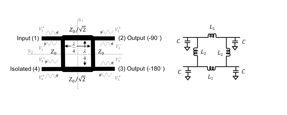
A special type of directional coupler is the Q-hybrid or branchline hybrid. This is a four-port device built from λ/4 microstrip segments or LC elements (lumped element equivalent) as shown in Figure 5. The relationship between incident and reflected voltage waves is given by the system scattering matrix (S4x4). This can be derived algebraically by considering four excitation modes such that each symmetry plane (s1 and s2 indicated in Figure 5) is a short circuit or open; and superposition of the four solutions [Ref.1 page 427-434]:
$$V_{4\times1}^{-}=S_{4\times4}V_{4\times1}^{+}, S_{4\times4}=\frac{-1}{\sqrt{2}}\begin{bmatrix} 0 & j & 1 & 0 \\j & 0 & 0 & 1\\1 & 0 & 0 & j\\0 & 1 & j & 0 \end{bmatrix} [4] $$
Due to the fourfold symmetry, independently of which port is selected as input, the signals will be 90 degree out of phase at the output ports (ports on the opposite side of the input port) and no signal will be present at the isolated port (adjacent to the input port). In the MRI quadrature excitation setup described in Figure 1, the transmit signal is injected to port 1 of the hybrid to generate two equal amplitude (-3 dB) quadrature signals in port 2 and 3 (hybrid operating as a power splitter and phase shifter):
$$V_{2}^{-}=\frac{1}{\sqrt{2}}(-jV_{1}^{+} ) [5]$$
$$V_{3}^{-}=\frac{1}{\sqrt{2}}(-V_{1}^{+} ) [6]$$
In practice, any mismatched condition in port 2 and 3 will generate a signal reflected back to the isolated port 4 (terminated with R=Z0) .
During detection the quadrature signals are injected in port 2 and 3, and combined in port 4 (hybrid operating as a power combiner) :
$$V_{4}^{-}=\frac{1}{\sqrt{2}}(-V_{2}^{+} - jV_{3}^{+}) [7]$$
when there is a 90 degree phase delay between port 2 and port 3, signals are combined at port 4 and cancelled at port 1.
In practice, we can get the device's S matrix through RF bench measurements using a network analyzer.
Cable trap
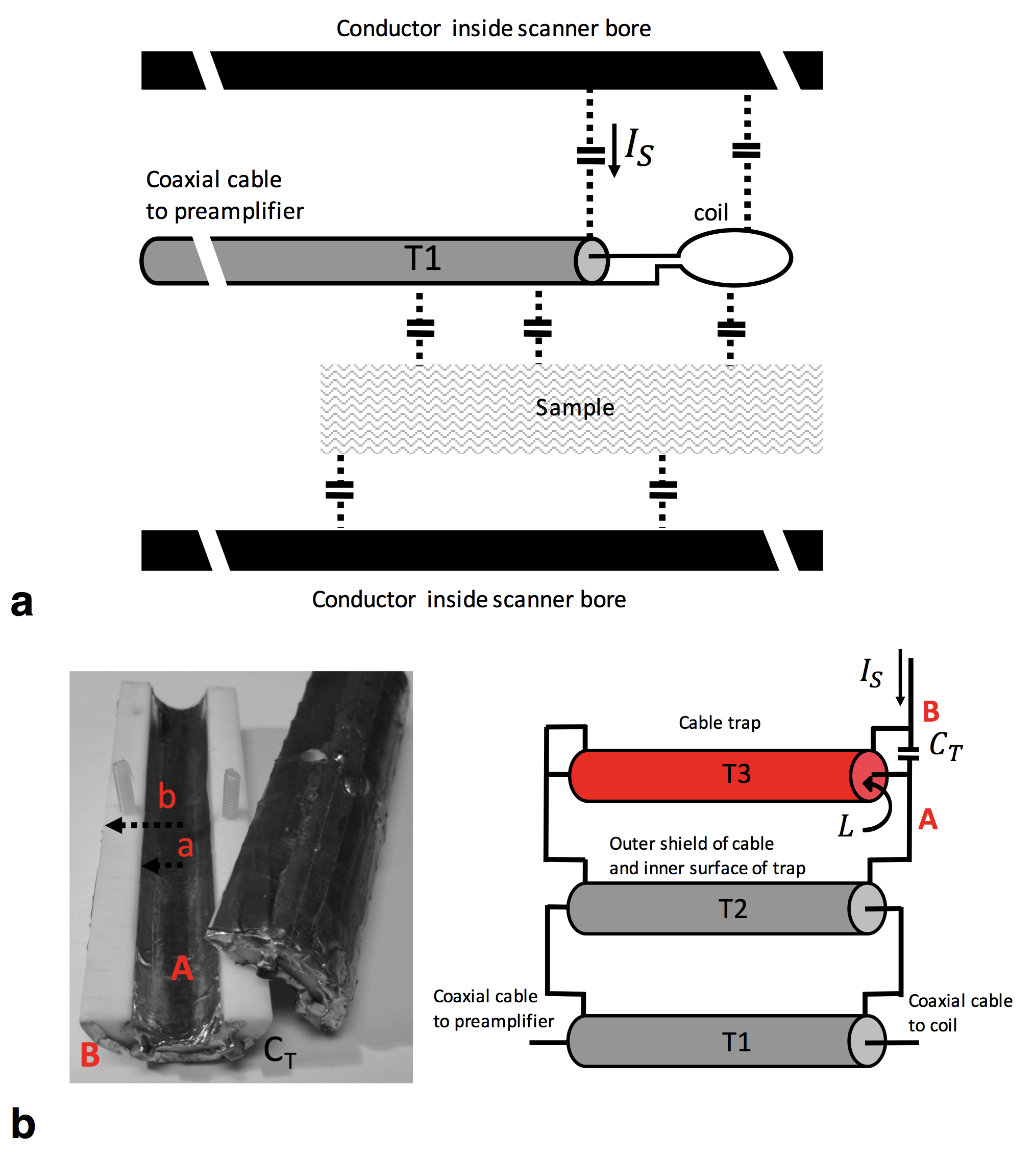
There are stray capacitances among the shield of coaxial connections, coil conductors, patient and the RF shield and coils inside the scanner bore (Figure 6a). During RF transmission, high voltages can be generated across these capacitances. These voltages drive common-mode currents on cable shields that can flow into the tissue and produce burns. Cable traps, designed based on the concept of resonance, are added to coaxial cables to introduce a large blocking impedance to suppress these shield currents. This is extremely important to ensure safety as well as to avoid cable cross talking when other coaxial connections are nearby. There are many types of cable traps. The simplest and most efficient way to construct one is to wind a portion of the coaxial cable into a solenoid shape. The shield inductance of this segment is resonated by an external capacitor soldered on the shield at both ends of the wound cable. One flexible trap design (based on the bazooka balun) is the floating cable trap (D.A. Seeber, et al. Concepts in Magn Res 2004; 21B;26–31). This trap can be easily clamped onto coaxial cables without need of soldering onto the cable shield. The trap is a TL formed by two halves of concentric copper layers coated on the outside and inside of a cylindrical form (of length d) made of a low dielectric insulator (like Teflon) to reduce the TL shunt capacitance (Figure 6b). A tuning capacitor is added between the inner and outer diameter of the cable trap to resonate the equivalent TL inductance. The coaxial cable and cable trap can be modeled as three interconnected TLs (Figure 6b). The shield current is blocked by the resulting high impedance of the parallel LC tank now formed by the total TL inductance of the trap and the external capacitor:
$$L=\frac{\mu}{2\pi}\ln\left(\frac{b}{a}\right)\left[H/m\right], C=\frac{2\pi\epsilon}{\ln\left(\frac{b}{a}\right)}\left[F/m\right] , \ for\ b >a \ and \ low \ \epsilon\rightarrow C_{T}\sim\frac{1}{(2\pi f)^2L\ d} [5] $$
In practice, tuning of the floating trap is also performed by adjusting the gap between the two halves of the trap which changes the mutual coupling (M) between them and affects the TL equivalent inductance.
Discussion
This presentation will focus on TL concepts and how these concepts are used in the design of the different interconnecting devices located in the transmit and the receive chains. Conventionally in MRI the RF signal travels along these chains through coaxial connections. However, the complexity of these connections (cabling layout, coupling and cable trap construction) increases with the number of transmit and/or receive channels. Therefore there are ongoing research efforts to replace coaxial connections by optical links or wireless communications. Miniaturization of the electronics is another important factor at the time of construction of high density arrays. To this end, TL segments are replaced by their lumped element equivalent. However a discrete component implementation becomes difficult when the MR frequency falls in the ultra-high frequency range (300 MHz-3 GHz). Finally, new RF approaches have been presented that eliminate the need of some of the conventional interconnections inserted between the RFPA and the coil, and between the coil and the RX RFA. I will discuss these non-conventional approaches further during the last part of my presentation.Acknowledgements
To my colleagues from the LFMI group for feedback received during the preparation of this syllabus contribution.References
Recommended Books
[1] R. E. Collin, Foundations for Microwave Engineering, 2nd ed. IEEE Wiley-Interscience, 2000
[2] J. C. Freeman, Fundamentals of Microwave Transmission Lines, John Wiley & Sons, Inc., 1996.
[3] T. H. Lee, Planar Microwave Engineering. Cambridge University Press, 2004.
[4] B. C. Wadell, Transmission Line Design Handbook. Artech House, Boston, 1991.
[5] D. M. Pozar, Microwave RF Engineering. 3rd ed, John Wiley & Sons, Inc., New York, 2005.
Figures