Principle of Electrical Properties Mapping
1Centre for Image Sciences, UMC Utrecht, Utrecht, Netherlands
Synopsis
This study gives an overview of the principles of Electrical Properties Tomography. The aim is to introduce researchers new to EPT in the basic EPT reconstruction principles, EPT artifacts and new directions.
It reviews Helmholtz based reconstruction, B1+ phase and transceive phase, boundary errors of EPT, forward vs inversion based EPT reconstruction and the synergy of EPT at high fields.
Objectives
- Obtain knowledge of various EPT reconstruction frameworks and understand their strengths and weaknesses.
- Understand the assumptions behind transceive approximation and methodologies to obtain direct B1+ phase.
- Understand the nature of reconstruction error at tissue boundaries
- Understand the differences between forward and inverse EPT approaches.
- Understand the performance of EPT for increasing field strength.
Introduction
Electrical Properties Tomography seeks to reconstruct the electrical conductivity and dielectric permittivity of human tissue from MRI based measurements of the B1+ transmit fields. The earliest attempt is the study by Haacke et al. but due to “spurious phase effects” was unable to demonstrate the feasibility [1]. Wen [2] showed first experimental results in 2003 but systematic research on socalled Electrical Property Tomography (EPT) only began in 2009 with the study by Katscher et al. [3] Since then the topic has gained traction and numerous studies have been published focusing mainly on acquisition and reconstruction aspects of EPT[4-8]. More recently more applications oriented papers have been published. In this educational talk some of the underlying principles of EPT, key electromagnetical aspects and assumptions and recent technical progress on EPT will be discussed.Helmholtz based Electrical Properties Tomography
Helmholtz based Electrical Properties Tomography
Most of the published EPT approaches are based on the so-called full Helmholtz wave equation: $$ -\triangle \overrightarrow{B}=\mu_{0}\omega k\overrightarrow{B}+\frac{\triangledown k}{k}\left(\triangledown\times \overrightarrow{B}\right)$$
which can be defined for a time-harmonic, source free magnetic field B=(Bx, By, Bz) and a complex permittivity (k=ωε-iσ) at an angular frequency ω. The second term in this wave equation couples different magnetic field components at regions where EP transitions occur. As this equation is valid for each Cartesian component, a similar equation can be drafted also for the positive circularly polarized component B1+ = (Bx + iBy)/2. A so-called truncated Helmholtz equation (eq. 2) can be formulated for the B1+ field for areas where gradient in k is zero, i.e. a piece-wise constant medium is assumed:$$-\triangle B_{1}^{+}=\mu_{0}\omega k B_{1}^{+}$$
With this truncated Helmholtz equation the complex permittivity k can be easily isolated. Unfortunately, several fundamental and technical issues complicate matters. These will be described in more detail below.
The transceive approximation
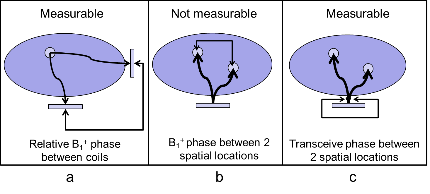
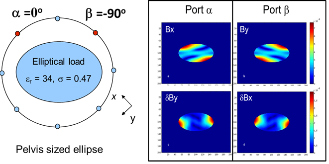
The transceiver phase approximation. Contrary to e.g. parallel transmission where the relative B1+ phase between different coil channels need to be mapped for proper RF shimming (see Figure 1a ) ,the B1+ phase required in EPT is the B1+ phase difference between two spatial location (See Figure 1b). However, in an MRI experiment, the radiofrequency field weighs into the signal formulation through the transmit field B1+ as well as the coil’s receive sensitivity, the B1- field. Therefore the total RF related signal phase arises from the phase of the B1+ transmit and B1- receive fields (See Figure 1c). We can define this phase as the socalled transceiver phase:$$\phi_{0}=\frac{\left(\phi_{+}+\phi_{-}\right)}{2}$$ where $$$\phi_{+}$$$ and $$$\phi_{-}$$$are the phase of the B1+ and B1- phase respectively. An often applied approximation in EPT, first introduced by Wen [2] called the transceiver phase approximation $$\phi_{+}\approx\frac{\phi_{0}}{2}$$We can analyze the physical rationale behind the transceive phase approximation by analyzing the B1+ transmit field and B1- receive field in more detail. In this analysis we assume for simplicity purpose that the transmission and reception takes place through the body coil (BC). Note that often a reception is performed through dedicated receiver array. However, when one applies receive field bias removal by a complex division by the receiver array’s sensitivity pattern, the effective receive field that enters is again the receive field of the body coil. This is the result of the way receiver array’s sensitivity pattern are typically determined. Typically, an image of a low flip GRE sequence recorded by the receiver array, is divided by an identical image recorded by the body coil. Assuming the body has a homogeneous receive field, this should result in a map of the receiver’s array sensitivity pattern. The body coil is typically of birdcage design and its two orthogonal channels are driven in quadrature. To be able to explain the principle of the transceive phase approximation, we follow the formulation of Overall et al, in the designation of the transverse magnetic field component for a quadrature birdcage coil. If we assume port $$$\alpha$$$ has an incident transverse magnetic field along the x-direction, the interaction of the incident field with the object results in an effective magnetic field $$$B_{x}^{\alpha}$$$ in the primary direction and a secondary field $$$\delta B_{y}^{\alpha}$$$ in the y-direction. This secondary field appears due to scatter currents in the objects (e.g. eddy currents). For port $$$\beta$$$, a similar formalism holds and we denote the primary field by $$$B_{y}^{\beta}$$$ and the secondary field $$$\delta B_{x}^{\beta}$$$. Assuming that a phase shift –i is applied in transmit to port $$$\beta$$$ in quadrature, the total transmit B1+ field $$$ B_{1}^{+}(_{quadTx})$$$ is given by:$$B_{1}^{+}(_{quadTx})=\frac{B_{x}^{\alpha}+B_{y}^{\beta}}{2}-i\left(\frac{\delta B_{x}^{\beta}-\delta B_{x}^{\alpha}}{2}\right)=K-iL$$ where we have denoted the term related to primary fields by K and the term related to the secondary field by L. Similarly, in receive mode a phase shift +i is applied to port $$$\beta$$$ , and the total receive field $$$ B_{1}^{-}(_{quadRx})$$$ is given by: $$B_{1}^{+}(_{quadRx})=\frac{B_{x}^{\alpha}+B_{y}^{\beta}}{2}+i\left(\frac{\delta B_{x}^{\beta}-\delta B_{x}^{\alpha}}{2}\right)=K+iL$$ Substituting these equations into the transceive phase we see that the only possibility for the transceive phase to reflect the B1+ phase is by setting the term L related to the secondary field equal zero. In that case, the transceive phase is indeed: $$$\phi_{+}=\frac{\phi_{0}}{2}$$$ This analysis demonstrates that the transceive phase approximation assumes the term L to zero. Physically, this can be achieved in a situation where the secondary fields are negligible which is generally the case for low field strengths (£ 1.5 T) and low conductive objects. Another possibility is that the secondary fields of channels a and b cancels each other over the objects which sets certain requirements with respect to their mutual amplitude and phase and therefore their position with respect to object. Such a situation is achieved for a spherical or cylindrical object placed symmetrical with respect to the ports.
For an elliptical object which is a more realistic approximation for anatomies such as the head, some caution should be respected. This is further illustrated in the figure 2 for a 7T quadrature birdcage coil. Given typical diagonal location of the ports $$$\alpha$$$ and $$$\beta$$$ of birdcage with respect to the major and minor axes of the ellipse, a mirror symmetry is apparent. It is observed that the secondary fields are minimal on the major and minor axis. Thus, given this mirror symmetric placement of the ports with respect to the ellipse, we see that the transceive phase approximation typically holds in the center of the ellipse but its approximation will deteriorate in more peripheral regions, especially in diagonal regions. For human anatomies such as the head or the pelvis, the ellipse is of course a first order approximation. Still, similar considerations have shown to hold for these anatomical regions[10,11].
An additional consideration in the validity of the transceive phase approximation is the effect of field strength A study by Van Lier et al. [12] has shown that in generally the transceive phase approximation remains fairly valid in the head at 3T, but a 7T is no longer valid and leads to erroneous conductivity and permittivity reconstructions (see figure 3 above). In the human abdomen and pelvis the approximation already deteriorates at 3T as the larger dimensions approach the “optical” wavelength. In general, one can state that the attractive feature of the transceive phase approximation is that it enables EPT with standard radiofrequency hardware. However, its validity at field strengths higher than 3T is very limited. A relevant aspect to mention here is the so-called phase-only EPT. As observed by Wen et al, conductivity information is primarily derived from RF phase information. As shown in detail by Voigt et al. [13] . in cases where the gradients in the B1+ magnitude are negligible, the conductivity \sigma can be simply calculated by taking the Laplacian on the transceive phase, which is referred to as the phase-only EPT. As demonstrated below, the linearity of this phase based EPT enables the circumvention of the transceive phase approximation: $$\sigma=\frac{\phi_{0}}{2\mu_{0}\omega}=\frac{\left(\phi_{+}+\phi_{-}\right)}{2\mu_{0}\omega}=\frac{\sigma}{2}+\frac{\sigma}{2}$$
In recent years various groups have shown ways to access directly the B1+ phase. An approach based on Gauss’ law was published by Zhang et al [14] that replaced the transceive approximation by the assumption that the gradients in Hz are negligible. For high field this might be advantageous as one can manage the validity of this assumption through proper RF coil design. Other methodologies are generally based on the fact that several transmit (Tx) channels are available and each Tx channel should result in identical EPT reconstructions. This situation is often the case for 7T where parallel transmit setups are quite common. A first study exploiting this concept was by Zhang et al. calling it the “Dual excitation algorithm” of [15], where it was applied to the EPT boundary problem. Later [16, 17], this concept was used to isolate the receive phase (common for all TX channels) and facilitating absolute H+ phase maps. The approach presented by [Marques14] differentiates itself by reconstructing EP maps based solely on relative sensitivity maps of receive coils. This has the advantage that (in contrast to map TX coil sensitivities) all coil sensitivities can be mapped simultaneously in a fast single scan, and thus, the method was dubbed “Single Acquisition Electrical Properties mapping” (SAEP). A more generalized methodology was presented by [18,19] aiming to reconstruct even more electromagnetic quantities by considering the general case of anisotropy and gradient in EPs, called (generalized) “Local Maxwell Tomography” (LMT).
Boundary error
A key disadvantage of the truncated Helmholtz reconstruction framework is that it fails at dielectric interfaces because of the invalidity of the reconstruction model. At the location of the interfaces, the full Helmholtz equation should be used. The error, this invalidity creates, has been investigated by several authors. Recently more advanced EPT reconstruction frameworks which take into consideration this boundary term have been presented. A framework for EPT, called gradient-based Electrical Properties Tomography (gEPT) was introduced by Liu et al.[20]. It is based upon the full Helmholtz equation, thus including gradients in electrical properties (Eps) at tissue boundaries. Assuming that derivatives of dH±/dz are much smaller dH±/dx, dH±/dy , which is generally true for most coil types in the central imaging zone, they demonstrated that all three spatial EP gradients could be reconstructed from multi-channel transceiver H+ or H- field data . By subsequent spatial integration starting from certain seed points with known EP, the complete EP distribution can be recovered. Furthermore, the gEPT framework is free of any phase assumptions. In their work, the authors present 7T brain results that demonstrate the superiority of their gEPT approach over conventional EPT. Another approach which takes into consideration also gradients of conductivity at interfaces has been presented by Gurler et al. [21] This approach is based on transceive phase data and is intended for conductivity reconstruction only. The final reconstruction requires the solution of a partial differential equation forming a convection-reaction-diffusion equation where only the transceive phase appears in the equation. This equation is solved with a finite difference scheme on a grid. In this approach also several assumptions are being made: (a) |\triangledown B_{1}^{+}| \approx0, |\triangledown B_{1}^{-}| \approx0 , (b) all derivatives with respect to Hz are ignored and (c) \sigma >> \omega \epsilon. Assumptions (a) and (c) are also underlying the “phase-based conductivity imaging” and lead to over-estimations of conductivity (e.g., approximately 20% for white and gray matter at 3T). As said, the above mentioned reconstruction framework try to address the model invalidity of conventional EPT at tissue boundaries. However, in addition to the resulting artifacts, also the numerical approximation of spatial derivatives places an important role. In practice, first and second order derivatives are computed by convolving the reconstructed MR image on a discretized grid with finite difference schemes (kernels). The problem is that at tissue boundaries, the kernels used to approximate spatial derivatives include voxels belonging to regions with different electrical properties resulting in erroneous reconstructions. This typically leads to under and over shooting of the reconstructed conductivity and permittivity values at boundaries. The spatial extent of these erroneous regions can be decreased by reducing the differentiation kernel, see Fig. 4 for an illustration of this effect on simulated B1+ data of a phantom consisting of various conductivity compartments. However, since the differentiation makes EPT very susceptible to noise on B1+ data, typically a relatively large spatial differentiation kernel has to be used resulting in severe blurring in final reconstructions.Forward vs Inversion based reconstruction approaches
All the described EPT reconstruction framework can be categorized as forward based approaches, i.e. operations are performed on measured B1+ field data which suffers of course of the presence of noise. An alternative approach, as proposed by various studies [22-24], is a general inverse method, running “forward” from tissue EPs to (measurable and non-measurable) fields. Thus, this approach fits a model of the EP distribution to the B1 field avoiding any differentiation on the measured B1 field. The fitting takes places by iteratively minimizing a large system (over all voxels) of non-linear equations with iterative methods such as conjugate gradient methods. The key advantage is that differentiations on measured noisy B1+ data are avoided. However, this comes at the expense of increasing computation costs due slow convergence and scale of the optimization problem. Furthermore, this type of non-linear inverse approaches that work by iterative optimization always have the risks of ending up in local minima. However, some of these approaches have shown some good results with excellent performance at tissue boundaries.Applications at high fields.
EPT derives information of local EP from the local RF field curvature. Since the RF field curvature increases at high field due to a higher wavenumber, in addition to increased signal-to-noise of high static fields, the sensitivity of EPT is expected to increase with field strength. The study of Van Lier et al [12], demonstrated this aspect clearly. Using similar coils setups at 1.5, 3 and 7T they were able to show empirically that the sensitivity for conductivity scales approximately linearly with field strength, while the sensitivity to permittivity even scaled quadratically. This aspect was worked out in more detail by Lee et al [25], demonstrating clearly the synergy of EPT with increasing field strength. Of course a difficulty at higher field strength is that some of the assumptions of conventional EPT such as the transceive phase approximation start to break down. Fortunately, the recent new reconstruction frameworks such as gEPT have found mitigation strategies for this issue, and it seems that the route of successful development of EPT at high field lies open.Conclusions
EPT is a relatively young MRI technique that can non-invasively probe electrical properties of tissues. This has potential applications in RF safety assessment (local SAR determination) and more importantly, offers a new endogenous contrast to characterize tissue pathologies. The first EPT reconstruction framework was based upon the truncated Helmholtz equation which fails at tissue boundaries and is susceptible to noise amplification through its 2nd finite differentiation. Recently, more sophisticated approaches such as gEPT have been presented that address the boundary artefact. A new trend is the switch to inversion approach as compared to the forward approaches. These type of approaches avoid differentiation on measured noisy B1+ field data and are more flexible in their formulation allowing e.g. the inclusion of regularization. Finally, in addition to improved reconstruction techniques, much gain in terms of sensitivity can be achieved by switching to higher field strengths.Acknowledgements
The authors thank Rob Remis and Ulrich Katscher for the open scientific exchange on EPT that helped to shape this abstract.References
- E. M. Haacke, et al. , “Extraction of conductivity and permittivity using magnetic resonance imaging,” PMB vol. 36,no. 6, pp. 723–734, 1991.
- H. Wen, “Non-invasive quantitative mapping of conductivity and dielectric distributions using the RF wave propagation effects in high field MRI,” in Medical Imaging: Physics of Medical Imaging, vol. 5030 of Proceedings of SPIE, pp. 471–477, February 2003.
- U. Katscher et al. “Determination of electrical conductivity and local SAR via B1 mapping,” IEEE Transactions on Medical Imaging, vol. 28, pp. 1365–1374, 2009.
- A. L. van Lier et al. “B1 phase mapping at 7T and its application for in vivo electrical conductivity mapping, ”MRM, vol. 67, pp. 552–561, 2012.
- Zhang X et al. Imaging Electric Properties of Biological Tissues by RF Field Mapping in MRI. IEEE Trans Med Imag 2010;2:474-481.
- Gurler et al. . Gradient-based electrical conductivity imaging using MR phase. MRM. 2016 Jan 13
- Seung-Kyun Lee et al. . Tissue Electrical Property Mapping from Zero Echo-Time Magnetic Resonance Imaging. IEEE Trans Med Imaging. 2015 Feb;34(2):541-50
- Marques et al. . Single acquisition electrical property mapping based on relative coil sensitivities: A proof-of-concept demonstration. MRM. 2014 Aug 5
- William R. Overall, John M. Pauly, Pascal P. Stang, and Greig C. Scott Ensuring Safety of Implanted Devices Under MRI Using Reversed RF Polarization MRM 64:823–833 (2010)
- Van Lier AL, Brunner DO, Pruessmann KP, Klomp DW, Luijten PR, Lagendijk JJ, van den Berg CA. B1(+) phase mapping at 7 T and its application for in vivo electrical conductivity mapping. Magn Reson Med. 2012 Feb;67(2):552-61
- Balidemaj E, van Lier AL, Crezee H, Nederveen AJ, Stalpers LJ, van den Berg CA. Feasibility of electric property tomography of pelvic tumors at 3T. Magn Reson Med. 2015 Apr;73(4):1505-13
- Van Lier AL, Raaijmakers A, Voigt T, Lagendijk JJ, Luijten PR, Katscher U, van den Berg CA. Electrical properties tomography in the human brain at 1.5, 3, and 7T: a comparison study. Magn Reson Med. 2014 Jan;71(1):354-63
- Voigt T, Katscher U, Doessel O. Quantitative conductivity and permittivity imaging of the human brain using electric properties tomography. Magn Reson Med. 2011 Aug;66(2):456-66
- Zhang X, Van de Moortele PF, Schmitter S, He B. Complex B1 mapping and electrical properties imaging of the human brain using a 16-channel transceiver coil at 7T. Magn Reson Med. 2013 May;69(5):1285-96
- Zhang X, Zhu S, He B. Imaging Electric Properties of Biological Tissues by RF Field Mapping in MRI. IEEE Trans Med Imag 2010;2:474-481.
- Katscher U, Findeklee C, Voigt T. B1-based specific energy absorption rate determination for nonquadrature radiofrequency excitation. Magn Reson Med. 2012 Dec;68(6):1911-8.
- Liu J, Zhang X, Van de Moortele PF, Schmitter S, He B. Determining electrical properties based on B(1) fields measured in an MR scanner using a multi-channel transmit/receive coil: a general approach. Phys Med Biol. 2013;58(13):4395-408
- Daniel K. Sodickson, Leeor Alon, Cem Murat Deniz, Ryan Brown, Bei Zhang, Graham C. Wiggins, Gene Y. Cho, Noam Ben Eliezer, Dmitry S. Novikov, Riccardo Lattanzi, Qi Duan, Lester A. Sodickson, and Yudong Zhu. Local Maxwell Tomography Using Transmit-Receive Coil Arrays for Contact-Free Mapping of Tissue Electrical Properties and Determination of Absolute RF Phase. Proc. Intl. Soc. Mag. Reson. Med. 20 (2012) 387
- Sodickson D. K. Alon L. Deniz CM Ben-Eliezer N, Cloos M, Sodickson LA, Collins CM, Wiggens GC, Novikov DS. Generalized Maxwell tomography for mapping of electrical property gradients and tensors. Proceedings of 21st Annual Meeting of ISMRM, Abstract 4175, Salt Lake City, USA, 2013.
- Jiaen Liu, Xiaotong Zhang, Sebastian Schmitter, Pierre-Francois Van de Moortele and Bin He. Gradient-Based Electrical Properties Tomography (gEPT): A Robust Method for Mapping Electrical Properties of Biological Tissues In Vivo Using Magnetic Resonance Imaging. Magn. Reson. Med. 74:634–646 (2015)
- Gurler N, Ider YZ. Gradient-based electrical conductivity imaging using MR phase. Magn Reson Med. 2016
- Balidemaj E, van den Berg CA, Trinks J, van Lier AL, Nederveen AJ, Stalpers LJ, Crezee H, Remis RF. CSI-EPT: A Contrast Source Inversion Approach for Improved MRI-Based EPT. IEEE Trans Med Imag 2015;34:1788-96
- Borsic A, Perreard I, Mahara A, Halter RJ. An Inverse Problems Approach to MR-EPT Image Reconstruction. IEEE Trans Med Imaging. 2016 Jan;35(1):244-56.
- Kathleen M Ropella and Douglas C Noll. A Regularized Model-Based Approach to Phase-Based Conductivity Mapping using MRI. Magn. Reson Med 2016. ePub ahead of print.
- Lee SK, Bulumulla S, Hancu I. Theoretical Investigation of Random Noise-Limited Signal-to-Noise Ratio in MR-Based Electrical Properties Tomography. IEEE Trans Med Imaging. 2015 Nov;34(11):2220-32
- S. Mandija, A. Sbrizzi, A.L.H.M.W. van Lier, P. Luijten, C.A.T. van den Berg, Artifacts Affecting Derivative of B1+ maps for EPT Reconstructions, Proceeding of the 24th Annual Meeting, Singapore, (2016), 2989
Figures