Synopsis

The basic principles of NMR are discussed based on classical concepts like compass needles, bar magnets, precession and electromagnetic induction. More advanced topics such as chemical shift, scalar coupling, T1 and T2 relaxation and basic MR sequences are also covered.

1. Classical magnetic moments

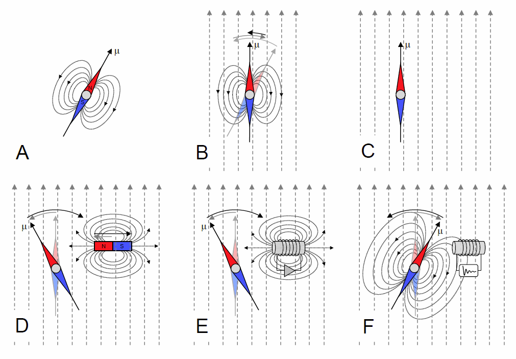
Many aspects of magnetic resonance (MR) can be understood without resorting to quantum mechanics by using classical, macroscopic analogs such as a compass, composed of a magnetized needle (1). As with all magnets, the compass needle is characterized by a magnetic north and south pole from which the magnetic field lines exit and enter the needle, respectively (Fig. 1A). The magnetic field lines shown in Fig. 1A can be summarized by a magnetic moment, µ, describing both the amplitude and direction. In the absence of an external magnetic field the compass needle has no preference in spatial orientation and can therefore point in any direction. When placed in an external magnetic field, such as the Earth’s magnetic field, the compass needle experiences a torque (or rotational force) that rotates the magnetic moment towards a parallel orientation with the external field (Fig. 1B). As the magnetic moment ‘overshoots’ the parallel orientation, the torque is reversed and the needle will settle into an oscillation or frequency that depends on the strengths of the external magnetic field and the magnetic moment. Due to friction between the needle and the mounting point the amplitude of the oscillation is dampened and will ultimately result in the stable, parallel orientation of the needle with respect to the external field (Fig. 1C) representing the lowest magnetic energy state (the anti-parallel orientation represents the highest magnetic energy state).

The equilibrium situation (Fig. 1C) can, besides mechanical means, be perturbed by additional magnetic fields as shown in Fig. 1D. When a bar magnet is moved towards the compass, the needle experiences a torque and is pushed away from the parallel orientation. When the bar magnet is removed, the needles oscillates as shown in Figs. 1B before returning to the equilibrium situation (Fig. 1C). However, if the bar magnet is moved back and forth relative to the compass, the needle can be made to oscillate continuously. When the movement frequency of the bar magnet is very different from the natural frequency of the needle the effect of the bar magnet is not constructive and the needle never deviates far from the parallel orientation. However, when the frequency of the bar magnet movement matches the natural frequency of the needle the repeated push from the bar magnet on the needle is constructive and the needle will deviate increasingly further from the parallel orientation. When the bar magnet has a maximum effect on the needle, the system is in resonance and the oscillation is referred to as the resonance frequency. A similar situation arises when pushing a child in a swing; only when the child is pushed in synchrony with the natural or resonance frequency of the swing set does the amplitude get larger. The bar magnet can be replaced with an alternating current in a copper coil as shown in Fig. 1E. The alternating current generates a magnetic field that can perturb the compass needle. When the frequency of the alternating current matches the natural frequency of the needle, the system is in resonance and large deviations of the needle can be observed with modest, but constructive ‘pushes’ from the magnetic field produced by the coil. The compass needle continues to oscillate at the natural frequency for some time following the termination of the alternating current (Fig. 1F). The compass needle creates a time-varying magnetic field that can be detected through Faraday electromagnetic induction in the same coil previously used to perturb the needle. The induced voltage, referred to as the Free Induction Decay (FID), will oscillate at the natural frequency and will gradually reduce in amplitude as the compass needle settles into the parallel orientation. Fig. 1 shows that the MR part of NMR can be completely described by classical means. It is therefore also not surprising that Bloch titled his seminal paper ‘Nuclear induction’ as the electromagnetic induction is an essential part of MR detection (2-4).

2. Nuclear magnetization

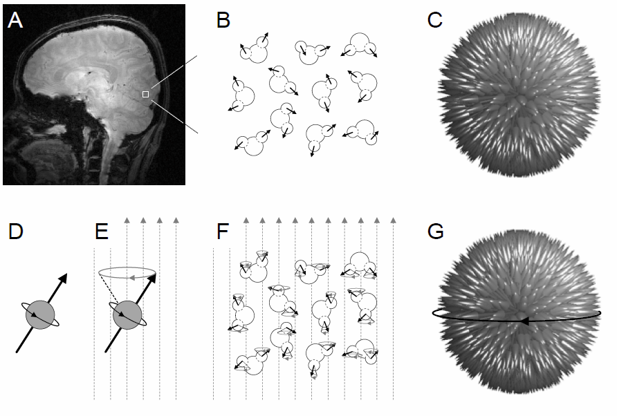
Any rotating object is characterized by angular momentum, describing the tendency of the object to continue spinning. Elementary particles like electrons, neutrons and protons have an intrinsic angular moment, or spin that is there even though the particle is not actually spinning. Electron spin results from relativistic quantum mechanics as described by Paul Dirac and has no classical analog. For the purpose of this introduction the existence of spin is simply taken as a feature of nature. Particles with spin always have an intrinsic magnetic moment. This can be conceptualized as a magnetic field generated by rotating currents within the spinning particle. This should, however, not be taken too literally as the particle is not actually rotating. Note that in the NMR literature spin and magnetic moment are used interchangeably. Protons are abundantly present in most tissues in the form of water or lipids. In the human brain a small cubic volume of 1 x 1 x 1 mm contains about 6 x 1019 proton spins (Fig. 2A/B). In the absence of an external magnetic field the spin orientation has no preference and the spins are randomly oriented throughout the sample (Fig. 2B). For a large number of spins this can also be visualized by a ‘spin-orientation sphere’ (Fig. 2C) in which each spin has been placed in the center of a Cartesian grid. Summation over all orientations leads to a (near) perfect cancelation of the magnetic moments and hence to the absence of a macroscopic magnetization vector.

Up to this point the nuclear magnetic moments behave similarly to the magnetic moments associated with classical compass needles. However, unlike compass needles nuclear magnetic moments have intrinsic angular momentum or spin which can be visualized as a nucleus spinning around its own axis (Fig. 2D). When a nuclear spin is placed in an external magnetic field (Fig. 2E) the presence of angular momentum makes the magnetic moment precess around the external magnetic field (Fig. 2E). This effect is referred to as Larmor precession and the corresponding Larmor frequency ν0 (in MHz) is given by

ν₀ = γB₀ (1)

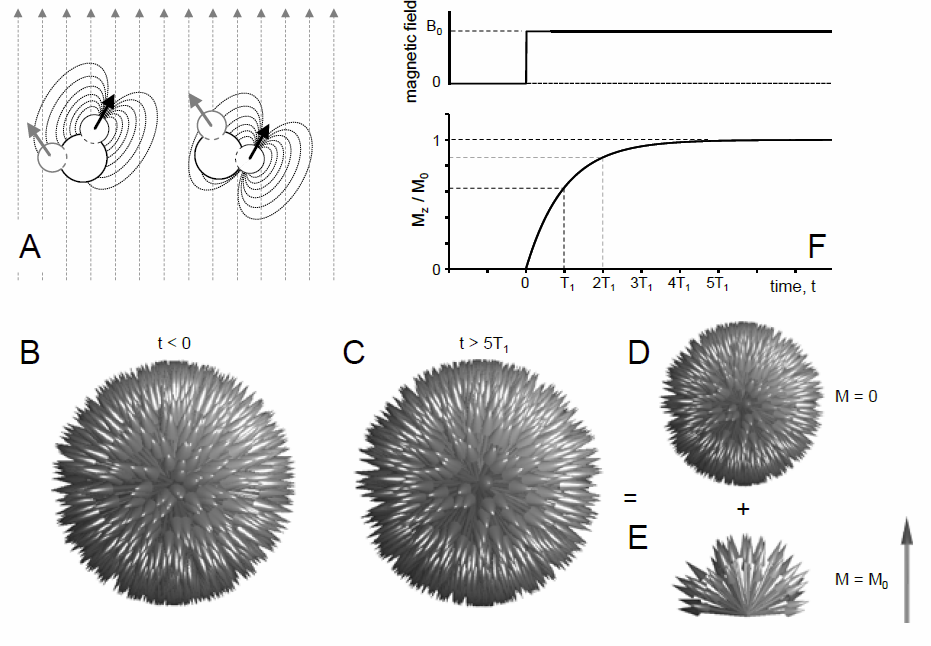
whereby γ is the gyromagnetic (or magnetogyric) ratio (in MHz/T) and B0 is the magnetic field strength (in T). The gyromagnetic ratio is constant for a given nucleus and equals 42.57 MHz/T for protons. When the protons depicted in Fig. 2B are subjected to an external magnetic field, every spin starts to precess around the magnetic field with the same Larmor frequency. As the orientation of the magnetic moment does (initially) not change, the spin-orientation sphere representation of Fig. 2C remains unchanged with the exception that the entire sphere is rotating around the magnetic field at the Larmor frequency. If Larmor precession would be the only effect induced by the external magnetic field, then NMR would never have developed into the versatile technique as we know it today. Fortunately, there is a second, more subtle effect that ultimately leads to a net, macroscopic magnetization vector that can be detected. The water molecules in Fig. 2B are in the liquid state and therefore undergo Brownian motion with a range of rotations, translations and collisions. As a result of Brownian movement the amplitude and orientation of the magnetic moment of one proton at the position of another moment changes over time (Fig. 3A). When the local field fluctuation matches the Larmor frequency it can perturb the spin orientation. These perturbations are largely, but not completely, random. The presence of a strong external magnetic field slightly favors the parallel spin orientation. As a result, over time the completely random spin orientation distribution (Fig. 3B) changes into a distribution that is slightly biased towards a parallel spin orientation (Fig. 3C). Visually, the spin distributions in the absence (Fig. 3B) and presence (Fig. 3C) of an external magnetic field look similar because the net number of spins that are biased towards the parallel orientation is very small, on the order of one in a million. The situation becomes visually clearer when the spin distribution is separated into spins that have a random orientation distribution (Fig. 3D) and spins that are slightly biased towards a parallel orientation (Fig. 3E). Adding the magnetic moments of Fig. 3D does not lead to macroscopic magnetization similar to the situation in Fig. 2G. However, adding the magnetic moments of Fig. 3E leads to a macroscopic magnetization vector parallel to the external magnetic field. As the external magnetic field only biases the spin distribution along its direction, the spin distribution in the two orthogonal, transverse directions is still random.

The microscopic processes detailed in Figs. 3A-E can be summarized at a macroscopic level as shown in Fig. 3F. In the absence of a magnetic field (t < 0) the sample does not produce macroscopic magnetization. When an external magnetic field is instantaneously turned on (t = 0), the macroscopic magnetization exponentially grows over time where it plateaus at a value corresponding to the thermal equilibrium magnetization, M0. The appearance of macroscopic magnetization can be described by

Mz (t) = M₀ − M₀ e^−t/T1 (2)

where T1 is the longitudinal relaxation time constant. At the time of the first NMR studies, little was known about T1 relaxation times in bulk matter. Both originators of NMR, Bloch and Purcell, were acutely aware that a very long T1 relaxation time constant could seriously complicate the detection of nuclear magnetism. As a precaution, Purcell used an exceedingly small RF field such as not to saturate the sample (5), whereas it is rumored that Bloch left his sample in the magnet to reach thermal equilibrium while on a skiing trip (6). Following the initial experiments it became clear that T1 relaxation time constants can range from milliseconds to minutes, with water establishing thermal equilibrium in seconds. Extraordinarily long T1 relaxation times may however have been the main reason for earlier, negative reports by Gorter (7, 8) on the detection of NMR in bulk matter. The longitudinal magnetization vector represents the signal that will be detected in an NMR experiment. However, the static, longitudinal magnetization is never detected directly as its small contribution would be overwhelmed by much larger contributions from magnetization associated with electron currents within atoms and molecules. Instead, the longitudinal magnetization is brought into the transverse plane where the precessing magnetization can induce signal in a receiver coil at the very specific Larmor frequency. The size of the longitudinal equilibrium magnetization and thereby the strength of the induced NMR signal is proportional to the number of spins that is biased towards a parallel orientation with the main magnetic field. The distribution of spin orientations and hence the bias in it can be calculated through the Boltzmann distribution which provides the probability P that a spin is in a certain orientation with an associated energy E according to

𝑃(𝐸)∝𝑒^{−𝐸/𝑘T} (3)

whereby k is the Boltzmann constant (1.38066 x 10–23 J/K) and T is the absolute temperature in Kelvin. Eq. (3) expresses the chance P of finding a particle with energy E in that state rather than in a random state determined by the available thermal energy of the environment (kT). For nuclear spins the energy limits are ±μB where μ is the magnetic moment and B the external magnetic field. The lower and higher energies correspond to nuclear spins parallel and anti-parallel to the external magnetic field respectively. Using either a continuous distribution of N spin orientations as shown in Fig. 3C or a quantized distribution the longitudinal equilibrium magnetization can be calculated from the Boltzmann distribution and is given by

\[M_0=N\frac{\gamma^2h^2B_0}{16\pi^2kT} \] (4)

with h representing Planck’s constant (6.62607 x 10–34 J.s). From Eq. (4) several important features concerning the sensitivity of NMR experiments can be deduced. The quadratic dependence of M0 on the gyromagnetic ratio γ implies that nuclei resonating at high frequency (see Eq. (1)) also generate the strongest NMR signals. Hydrogen has the highest γ of the commonly encountered nuclei, and has therefore the highest relative intensity. The linear dependence of M0 on the magnetic field strength B0 implies that higher magnetic fields improve the sensitivity. In fact this argument (and the related increase in chemical shift dispersion) has caused a steady drive towards higher magnetic field strength. Finally, the inverse proportionality of M0 to the temperature T indicates that sensitivity can be enhanced at lower sample temperatures. Obviously, the latter option is unrealistic for in vivo applications.

3. Nuclear induction

The orientation of a compass needle in Fig. 1 could be changed with an additional magnetic field perpendicular to the magnetic moment. Similarly, a second magnetic field, B1, is used to change the orientation of the longitudinal magnetization, M0. Fig. 4A shows three spins extracted from the large spin population shown in Fig. 3. Each of the spins undergoes Larmor precession around the magnetic field on its own cone, dictated by the initial orientation of the magnetic moment. When a stationary magnetic field B1 is applied, the red spin rotates towards the transverse plane, whereas the orange spin rotates towards the longitudinal axis. However, at a time 1/(2ν0) (= 1.68 ns for 1H at 7 T) later the spins have precessed by 180° and now the red spin is rotated away from the transverse plane and the orange spin away from the longitudinal axis. It is thus clear that a static B1 field cannot rotate the spins as any rotation achieved during one half of a precession cycle is undone by the second half. In other words, the magnetic field B1 is not in resonance with the spins and its effect is therefore negligible. However, as shown for the compass needle in Fig. 1 the second magnetic field can have a large effect when its frequency matches the natural, or Larmor, frequency of the compass needle. Fig. 4C shows the same three spins in the presence of a rotating magnetic field B1 whose frequency equals the Larmor frequency. It follows that the angle between the magnetic moments and the magnetic field B1 is constant, leading to a coherent rotation towards the transverse plane. It should be noted that the magnitude of the rotating B1 magnetic field is typically 5 to 6 orders smaller than the static B0 magnetic field. In addition, it should be noted that NMR uses magnetic fields rotating at the RF frequency, not electromagnetic RF waves (9, 10). The electric component of electromagnetic RF waves is not relevant for NMR and proper RF coil design is aimed at minimizing its contribution.

At this point it should be mentioned that the secondary magnetic field B1 is typically not applied as a rotating magnetic field, but rather as a cosine-modulated magnetic field traversing between the +x and –x axes (Fig. 4D). However, a linear cosine-modulated magnetic field can be seen as the vector sum between clockwise and counter-clockwise rotating components (Fig. 4E). The counter-clockwise component can be ignored as it is not in resonance with the spins and therefore does not produce a coherent rotation, leaving just the clockwise rotating component to rotate the nuclear magnetic moments. Fig. 4F shows the thermal equilibrium magnetization M0 before the application of an RF pulse, separated out into the majority of randomly distributed spins that do not contribute to M0 (Fig. 4G) and the small number of spins that are biased towards a parallel orientation, thereby forming the macroscopic magnetization M0 (Fig. 4H). Fig. 4I-K show the situation immediately after the application of an RF pulse that is adjusted in length and amplitude to rotate M0 exactly 90°. Visually the spin-orientation spheres before (Fig. 4F) and after (Fig. 4I) the RF pulse appear similar. But since the entire sphere has been rotated by 90° the fraction of the spin population that was biased along B0 (Fig. 4H) is now biased along the y axis in the transverse plane (Fig. 4K). As each of the individual spins is precessing at the Larmor frequency, the total magnetization is also precessing at the same frequency and can be detected through electromagnetic induction in a nearby receiver coil.

Acknowledgements

References