Synopsis

This lecture will cover the basics of diffusion MRI. We will explore how diffusion in biological tissue serves as an in vivo microscope through its measurement with MRI by varying both diffusion gradient and the diffusion time t, the time over which the molecules diffuse. The concepts of q-space imaging, diffusion tensor imaging (DTI) and diffusion kurtosis imaging (DKI) will be covered, as well as other higher order diffusion methods (biophysical models versus representations). In addition, we will illustrate how varying the diffusion time t provides complimentary information about microstructural length scales.

Highlights

· Water molecules undergo random motion known as diffusion

· In biological tissue, the diffusion of molecules is altered by the presences of membranes and organelles, and varies with direction and diffusion time

· Diffusion MRI measures the diffusion properties (of NMR visible molecules) by varying the diffusion gradient and diffusion time t

· The diffusion tensor captures the Gaussian properties of the diffusion MRI signal

· High-order methods aim to describe the “beyond DTI” diffusion MRI signal mathematically or interpret it directly in terms of underlying microstructural features

Objectives

· Explore how the diffusion properties in biological tissue can be measured with MRI by both varying the diffusion gradient wave vector q and diffusion time t

· Comprehend the difference between diffusion signal representations and biophysical models

Methods

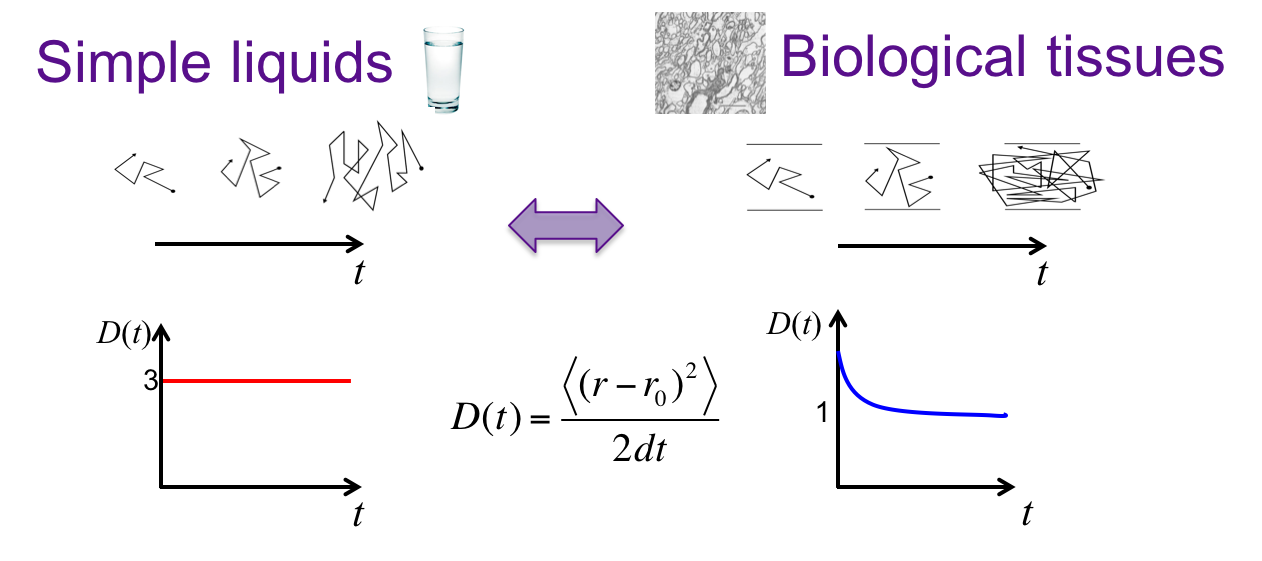
Water molecules undergo random motion due to thermal energy, called Brownian motion or diffusion. In a homogeneous medium such as water, the diffusion is the same in all directions (i.e. isotropic) with a diffusion displacement profile (a.k.a. diffusion propagator) characterized by a Gaussian distribution with a variance, i.e mean square displacement, growing linearly with time. The diffusion coefficient, defined as the mean square displacement over time, $$$D(t) \equiv \langle x^2(t)\rangle/2t$$$, is constant in this case (Fig. 1). In biological tissue, however, the diffusion becomes directionally dependent (i.e. anisotropic), and the diffusion coefficient will depend on time. Indeed, for increasing diffusion times, diffusing particles encounter gradually more restrictions (Fig. 1, thereby directly probing the tissue microstructure. The diffusion propagator is not Gaussian anymore.

The non-Gaussian diffusion signal as observed in biological tissue can be measured with MRI (Fig. 2 conventional Stejskal-Tanner sequence) by varying both the wave vector q (determined by gradient strength and direction) and the diffusion time t, the time over which the molecules diffuse. While both q and t are typically collectively grouped together as the diffusion weighting, b-value or b-matrix, we will explore both avenues here separately to illustrate their different specific sensitivities (Fig. 2: q-t graph).

Exploring q-space

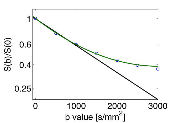
q-space imaging (QSI), pioneered by Stejskal, Tanner [1] and Callaghan [2], measures the diffusion signal as function of the gradient wave vector q, defined as: q = δg, where g is the gradient wave vector corresponding to the direction and magnitude of the diffusion gradient, and δ is the gradient pulse duration. (q is here analogous to the vector k which is at the basis of the MRI theory.) By applying pulse-field gradients, the diffusion MRI signal or propagator, S (q,t), becomes the spatial Fourier transform (in q) of the voxel-averaged diffusion propagator. Mathematically, the diffusion propagator admits a regular expansion of ln(S (q,t) ) in terms of b=q²t (in case of narrow pulse limit), a.k.a. the cumulant expansion [3], whereby the 1st and 2nd-order term yields the diffusion coefficient and kurtosis (Fig. 3).

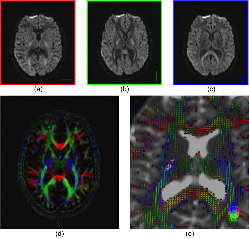
Diffusion tensor imaging (Fig. 4): At low diffusion weighting (bD<< 1/K) the diffusion signal can be well represented by the lowest-order term in Eq (2), $$$ln S \simeq –bD(t)$$$. The diffusion coefficient $$$D(t) \equiv \langle x^2(t)\rangle/2t$$$ is a measure of how fast mean squared molecular displacement grows with time. Since biological tissues such as white matter are anisotropic, this Gaussian part is, in general, a rank-2 diffusion tensor D, characterized by a $$$3\times3$$$ symmetric matrix with 6 independent parameters. The linear estimation problem of D, referred to as diffusion tensor imaging (DTI), has been solved by Basser et al in 1994 [4]. It requires measurements for at least one b ≠0 value (often set at 1000 s/mm² for brain) along at least six non-collinear directions in addition to the b = 0 (unweighted) image. The diffusion tensor is usually visualized by an ellipsoid, whereby the axes of the ellipsoid coincide with the eigenvectors and the corresponding eigenvalues are taken as radii. A number of scalar indices can be derived from the diffusion tensor, including the widely used mean diffusivity (MD) and fractional anisotropy (FA).

DTI is most commonly used to visualize white matter anisotropy and has shown to be very useful in clinical application [5, 6]. Though, it is important to note that DTI estimates only the lowest-order term of the cumulant series (2), thereby probing the Gaussian properties of the propagator, yielding no information about higher-order terms, and practically one should always choose the b-range such that the higher-order terms do not bias the estimation of D. Similarly, the diffusion tensor is not able to accurately describe fiber geometries in voxels containing multiple fiber tracts in multiple directions, e.g., crossing fibers.

Diffusion kurtosis imaging extends conventional DTI by estimating the kurtosis of the water diffusion probability distribution function based on the diffusion signal acquired at slightly higher diffusion weighting (b-value ≤ 2000 s/mm²). In case of diffusion anisotropy, DKI requires the introduction of a rank-4 diffusional kurtosis tensor in addition to the rank-2 diffusion tensor used in DTI. The linear estimation problem of both the diffusion and kurtosis tensors, via the expansion up to b², referred to as diffusion(al) kurtosis imaging (DKI) , has been solved by Jensen et al in 2005 [7]. The number of parameters is now 6 (diffusion tensor) + 15 (kurtosis tensor) = 21, hence at least two b ≠0 values (often set at 1000 and 2000 s/mm² for brain) for at least 15 non-collinear directions in addition to the b= 0 (unweighted) image are required. The weights for unbiased estimation of diffusion and kurtosis tensors for non-Gaussian NMR noise were recently proposed [8]. Qualitatively, a large diffusional kurtosis suggests a high degree of diffusional heterogeneity and/or microstructural complexity [9]. The extra information provided by DKI can also resolve intra-axonal fiber crossings and thus improve fiber tractography of white matter [10].

Signal representations versus biophysical models [11]: While both DTI and DKI are popular methods that empirically have shown sensitivity to pathological changes in the brain and body, it is important to note that both methods are examples of diffusion signal representations (i.e., convenient mathematical functions which fit the data well) and cannot be interpreted directly in terms of the underlying microstructure. To become specific to microstructure, many biophysical models for specific tissue types have been proposed, as will be discussed in the next lecture. These models have concrete assumptions about tissue parameters and have, per definition, limited range of applicability.

Exploring the time-axis

The unique advantage of diffusion MRI arises from the sensitivity of water diffusion to the tissue microstructure, and holds the promise of quantifying relevant length scales, such as the cell size and packing correlation length. Rather than by probing q space, where 1 μm diameter axons and dendrites require q values prohibitively large for in vivo human measurements, we propose to derive the relevant micrometer-level length scales by varying t. This formally amounts to a q ~ 0 measurement and is thereby clinically feasible. Since the diffusion coefficient in a given direction is a measure of the mean squared displacement, i.e. , we can vary the length scale probed by the water molecules by varying t. With increasing t, water molecules encounter more hindrances and restrictions to their diffusion paths (Fig. 1), such as cellular walls and myelin, and therefore the resultant measured diffusion coefficient will decrease [12-14]. The biophysical origin of observed time-dependence reflects the non-Gaussian nature, and thereby potentially enables novel microstructural contrasts, as recently demonstrated for time dependent diffusion observed in vivo in brain white matter [15].

Acknowledgements

Dmitry Novikov, Jelle Veraart and Valerij Kiselev.

References

1. E. O. Stejskal and J. E. Tanner, Spin Diffusion Measurements: Spin Echoes in the Presence of a Time-Dependent Field Gradient. The Journal of Chemical Physics, 1965. 42: p. 288.

2. Callaghan, P.T., C.D. Eccles, and Y. Xia, NMR microscopy of dynamic displacements: k-space and q-space imaging. Journal of Physics E: Scientific Instruments, 1988. 21(8): p. 820.

3. Kiselev, V., The cumulant expansion: an overarching mathematical framework for understanding diffusion NMR., in Diffusion MRI: Theory, Methods and Applications, D. Jones, Editor. 2010, Oxford University Press: Oxford.

4. Basser, P.J., J. Mattiello, and D. LeBihan, MR diffusion tensor spectroscopy and imaging. Biophysical Journal, 1994. 66(1): p. 259-267.

5. Behrens, T. and H. Johansen-Berg, Preface, in Diffusion MRI. 2009, Academic Press: San Diego. p. xi.

6. Jones, D.K., Diffusion MRI Theory, Methods and Applications. First ed. 2010: Oxford University press.

7. Jensen, J.H., et al., Diffusional kurtosis imaging: the quantification of non-gaussian water diffusion by means of magnetic resonance imaging. Magn Reson Med, 2005. 53(6): p. 1432-1440.

8. Veraart, J., et al., Weighted linear least squares estimation of diffusion MRI parameters: Strengths, limitations, and pitfalls. Neuroimage, 2013. 81: p. 335-346.

9. Jensen, J.H. and J.A. Helpern, MRI quantification of non-Gaussian water diffusion by kurtosis analysis. NMR in Biomedicine, 2010. 23(7): p. 698-710.

10. Lazar, M., et al., Estimation of the orientation distribution function from diffusional kurtosis imaging. Magnetic Resonance in Medicine, 2008. 60(4): p. 774-781.

11. Novikov D.S., Jespersen S.N., Kiselev V.G., Fieremans E. Quantifying brain microstructure with diffusion MRI: Theory and parameter estimation. preprint arXiv:1210.3014 [physics.bio-ph]

12. Mitra, P.P., et al., Diffusion Propagator as a Probe of the Structure of Porous Media. Physical Review Letters, 1992. 68: p. 3555-3558.

13. Novikov, D.S., et al., Revealing mesoscopic structural universality with diffusion. Proceedings of the National Academy of Sciences of the United States of America, 2014. 111(14): p. 5088-93.

14. Burcaw, L.M., E. Fieremans, and D.S. Novikov, Mesoscopic structure of neuronal tracts from time-dependent diffusion. Neuroimage, 2015. 114: p. 18-37.

15. Fieremans, E., et al., In vivo observation and biophysical interpretation of time-dependent diffusion in human white matter. NeuroImage, 2016. 129: p. 414-427.