Synopsis

This presentation is designed to give an overview of the building blocks of an MRI receive RF chain, starting with the local MRI coil going all the way to the image processor.

1. Introduction

This presentation is designed to give an overview of the building blocks of an MRI receive RF chain, starting with the local MRI coil going all the way to the image processor. Further information on this topic can be found in (1). This book contains a detailed introduction to MRI as well as other diagnostic imaging systems.

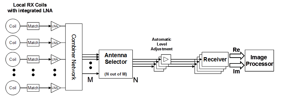
Figure 1 shows a typical receive chain consisting of the following building blocks:

• RF coils
• Detuning circuits
• Matching networks
• Low noise preamplifiers (LNAs)
• Combiner circuitry
• Coil cables and Baluns
• Antenna selector
• Automatic level adjustments
• Receivers

The purpose of the RF chain can be summarized as follows:

“Select and extract a set of MRI signals from a subset of local MRI coils in a patient save and user friendly manner, with high SNR and high linearity, and convert them from analog RF signals to digital complex k-space data.”

Some important parameters to characterize an RF receive chain are:

• Frequency
• Bandwidth
• Dynamic Range
• Noise figure
• Linearity
• Channel crosstalk
• Jitter
• Number of parallel RF channels
• Size of channel selector

2. Building blocks of the RF chain

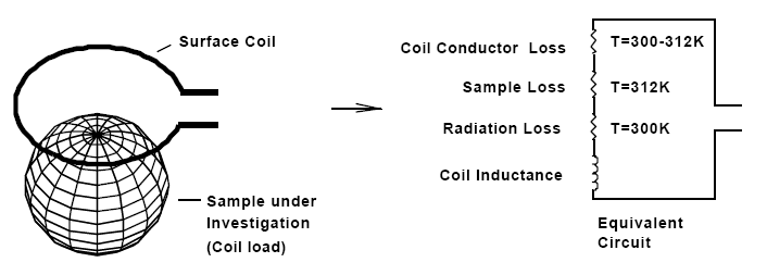
2.1. MRI coil including detuning, matching and LNA Figure 2 shows an MRI coil in the vicinity of a conductive sample and the associated equivalent circuit (2-5). As can be seen, the coil can be modeled as lossless inductor in series with a set of resistors that represent losses originating from coil conductor, sample and radiation. The resistance of a well-designed MRI coil under typical patient loading condition is mainly due to the patient tissue. This can be confirmed by resonating the coil and measuring the ratio of unloaded to loaded Q. A Q ratio of 5 or higher is a good indicator for a sensitive MRI coil.

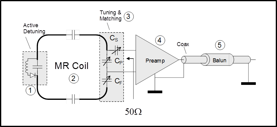
In order to extract the MRI signal from the coil with highest SNR possible, the coil impedance has to be transformed via a lossless transformation network to an impedance that insures minimum noise contribution from the connected low noise preamplifier (LNA). Typically, LNAs are optimized for a noise match impedance of 50 Ohms. Figure 3 shows the most important components of an MRI coil, which are detuning circuit, tuning and matching circuit, LNA and coil cable with one or more Baluns.

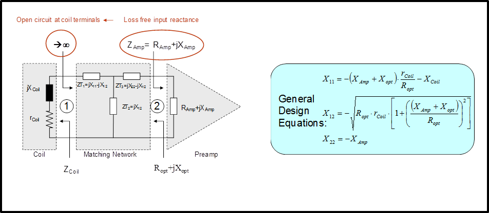
In array coil applications, the preferred method of matching coils to preamplifiers involves so called “isolating matching networks” (6). These networks serve two distinct purposes:

1. They transform the coil impedance to the desired noise match impedance (in this example 50 Ohms).
2. They do transform the preamp input reactance into a high impedance at the coil feed point.

The latter is important in order to reduce current flow on the coil and thus reduce the effect of inductive coupling on the measured coil input impedances of the array. Figure 4 shows such an isolating matching network including the formulas to calculate it.

Modern preamplifiers for MRI purposes have a noise figure of less than 0.5dB, i.e. the preamp reduces the available SNR by no more than 5%. These preamps also keep the linearity deviations to less than 1% over the full dynamic range (DR) of the MRI signal. This means, that the largest available MRI signal, typically created by 3D sequences with long TR, will not exceed the 0.1dB compression point of the preamplifier.

2.2 Combiner circuitry

Early array coils have been designed using linear (LP) or circular polarized (CP) coil elements. More recent developments are arrays of coils that use Mode Matrix or Eigencoil combiners (7, 8). These arrays consist of clusters of LP coil elements which are pre-combined to a set of mode signals. Figure 5 shows an example of a Mode Matrix combiner connected to a three-element coil cluster. The original coil signals R, M, L are fed into the Mode Matrix combiner and transformed to three new signals P, S, T. Eq. 1 shows the Mode Matrix for this specific example.

$$\left[\begin{array}{c} {P} \\ {S} \\ {T} \end{array}\right]=\underbrace{\left[\begin{array}{ccc} {\frac{1}{2} } & {-\frac{j}{\sqrt{2} } } & {-\frac{1}{2} } \\ {\frac{1}{\sqrt{2} } } & {0} & {\frac{1}{\sqrt{2} } } \\ {\frac{1}{2} } & {\frac{j}{\sqrt{2} } } & {-\frac{1}{2} } \end{array}\right]}_{{\rm Mode\; Matrix}} \cdot \left[\begin{array}{c} {R} \\ {M} \\ {L} \end{array}\right] [1]$$

The primary signal P is equivalent to the CP signal of a Loop-Butterfly combination, which is a common CP arrangement for planar coil arrays. The two remaining mode signals contain information from areas of the imaging region where the CP combination is not adequate to retrieve maximum SNR.

For non-parallel imaging applications, the CP Mode signal contains sufficient SNR to guarantee high image quality in the center of the imaging region. But when parallel imaging techniques like SENSE, SMASH or GRAPPA are used, the additional signals from Dual- or Triple Mode deliver the spatial information needed to support parallel image reconstruction (9-15). Dual- and Triple Mode signals can also be used for non-parallel imaging, where they will improve SNR in the peripheral image regions.

When using all three mode signals P, S, T, the combined array SNR is the same as when using the original signals R, M, L. However, the new signals P, S, T offer more flexibility to the user: Each of the original signals covers only a part of the FOV, while the mode signals cover the entire FOV. With mode signals, it is thus possible to scale the number of receiver channels between one and three depending on the application.

2.3 Coil cables and Baluns

As has been indicated in Figure 3, one or several “Balun” (balanced-to-unbalanced) structures have to be incorporated with the coil cable. These Balun structures minimize the flow of currents along the outside of the cable shield, thus prohibiting the cable to act itself as antenna. Suppressing shield currents is especially important during the sequence transmit phase, since excessive shield currents can lead to tissue heating and injuries. Therefore, care has to be taken to incorporate a sufficient number of these Baluns, also called “RF traps”, into the cable design and to make sure that these Baluns are properly tuned. Figure 6 shows the two most common Balun structures used with MRI coils.

2.4 Antenna selector

The antenna selector is a very important part of a modern workflow oriented MRI system. The antenna selector allows selecting a subset of the available MRI signals for further processing. The selection process is guided by the following parameters:

1. Origin of Signal Only those signals that come from within the region-of-interest (ROI) are selected
2. Mode of Operation Defines how many mode signals from a given set of coils are selected.
3. Number of available receiver channels Performance scanners are usually equipped with sufficient receivers. In economy scanners, the lower number of receivers leads to compromises between imaging speed and imaging quality.

Figure 7 shows an antenna selector which allows selecting up to 32 signals out of 76.

With continuous efforts of reducing cost and size of receivers, analog antenna selectors are about to become obsolete. Instead of preselecting RF channels, the scanner acquires and digitizes data from all available channels. Data selection, combination, and reconstruction is all done in the digital domain.

2.5 Automatic level adjustment

The dynamic range (DR) of a signal is defined as the margin between the maximum peak power of the signal (e.g. PS = –24dBm @ 1.5 T local coil LNA input) and the noise level (PN /Hz = -174 dBm/Hz at room temperature) The intrinsic dynamic range of the receive path must be considerably greater than the dynamic range of the signal in order not to sacrifice signal-to-noise ratio (SNR). In general, the limiting factor within the receive path is the intrinsic dynamic range of the Analog-Digital-Converter (ADC). A state-of-the-art 14 bit-ADC with 10 MHz bandwidth offers a dynamic range of approximately 153 dB/Hz, while the receive chain requires ~180dB/Hz. To overcome this limitation, automatic level adjustment are used to enhance the DR: The MR signal level is matched dynamically to the maximum level of the ADC by means of additional switchable gain elements or attenuators (Figure 8). Thus, the SNR of small MR signals will not be affected by the limited dynamic range of the ADC. State-of-the-art MR systems automatically adjust the MR signal level by one or more of these different methods:

1. Gain is fixed for the complete image acquisition time. The maximum MR level is forecasted based upon the coils used, sequence, slice thickness, and number of slices.
2. Gain is fixed for certain echoes of the image. Usually, only a few k-space lines (within the center of k-space) have maximum level. All other echoes could be collected with a higher gain level.
3. Gain is dynamically adjusted depending on the present MR signal level. This takes advantage of the fact that usually only the center portions of the centered k-space lines have the maximum level. Thus, only a very small percentage of the k-space values are affected by the limited ADC dynamic range. The dynamic switching could be based on a forecast, or by a level detection circuit.
4. Gain is continuously adjusted by means of an analog compressor, a matching expander after digitization restores the signal linearity.

Methods 2. - 4. require careful calibration of the hardware in order to avoid image artifacts.

2.6 Receivers

The MRI signal is a bandwidth limited signal centered around the main frequency of the magnet, which is ~64MHz for 1.5T and ~128MHz for 3T. We can look at the time domain MRI signal u(t) as a complex baseband signal F(t) modulated onto a carrier with frequency ω₀

$$\begin{equation} \label{GrindEQ__2_} u(t)=Re\left\{F(t)\cdot e^{j\omega _{0} t} \right\}=Re\left[F(t)\right]\cos \omega _{0} t-Im\left[F(t)\right]\sin \omega _{0} t \end{equation} [2] $$

The MRI receiver performs a quadrature demodulation of by multiplying the MR signal u(t) with an in-phase LO cos(ω₀t) and a quadrature LO sin(ω₀t)

$$\begin{equation} \label{GrindEQ__4_} u_{1} =u(t)\cos \omega _{0} t=\frac{1}{2} \left[Re\left[F(t)\right]+Re\left[F(t)\right]\cos 2\omega _{0} t-Im\left[F(t)\right]\sin 2\omega _{0} t\right] \end{equation} [3]$$

$$\begin{equation} \label{GrindEQ__5_} u_{2} =u(t)\sin \omega _{0} t=\frac{1}{2} \left[-Im\left[F(t)\right]+Im\left[F(t)\right]\cos 2\omega _{0} t+Re\left[F(t)\right]\sin 2\omega _{0} t\right] \end{equation} [4]$$

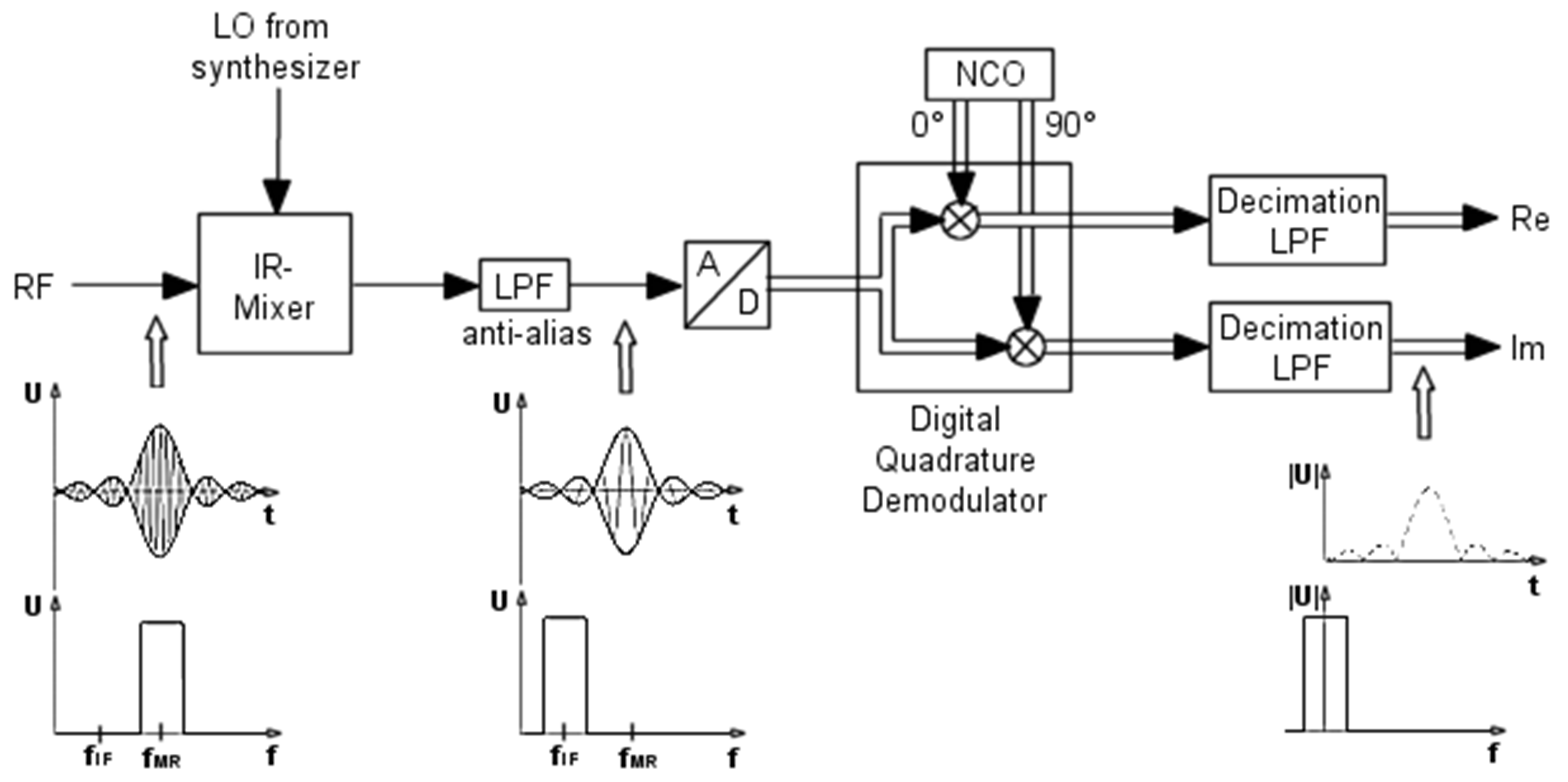
Afterwards, terms with 2ω₀ are suppressed by use of low pass filters (LPF). The filtered signals are representing the in-phase and quadrature components of the rotating frame signal F(t). These signals are fed as a discrete time series with time step T into the image processor. State-of-the-art receivers employ fully digital quadrature demodulators (Fig. 9).

The digitized signal u(t) is simultaneously multiplied with time discrete versions of cos(ω₀t) and sin(ω₀t), which are realized by a numerically controlled oscillator (NCO). The digital decimation LPF that follows, fulfills three tasks: Eliminating the 2ω₀ signal components, reducing the intrinsic (object) and artificial (noise figure of the Rx-path) noise, and reducing the noise contribution of the ADC.

Currently, the most common MR receiver topologies are

1. Intermediate Frequency (IF) Receiver
2. Direct Conversion (DC) Receiver

Figure 9 shows an IF receiver. With the help of an analog image rejection (IR) mixer, the MRI signal is converted to a lower intermediate frequency signal. Afterwards, the signal is fed via an anti-alias LPF into the ADC.

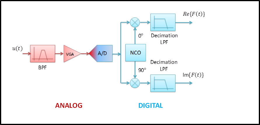
Figure 10 shows a topology for a direct conversion receiver. The main difference compared to the IF receiver is the absence of the IR mixer.

The sampling rate of the ADC has to satisfy Nyquist criterion for the bandwidth of the incoming signal, and not for the actual frequency, which can be significantly higher. In case of the DC receiver, it is common that the ADC sampling rate is lower than the MRI frequency. It just needs to be at least twice the bandwidth of the incoming signal to satisfy Nyquist. Higher ADC sampling rates will allow the use of wider bandpass filters, which are easier to obtain, but higher ADC sampling rates will also cause higher power consumption and dissipation.

If the ADC sampling rate is sufficiently high, a single ADC can be used to sample signals from several channels in a TDMA (time division multiple access) fashion. Phase coherency between channels needs to be guaranteed though, since MRI uses phase encoding for the image information.

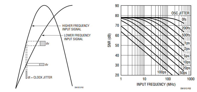
Sampling and mixing are closely related procedures. In both cases, errors from the mixing components will find their way to the output signal of the receiver. When sampling data, one of the mixing components is the sampling clock which will have some jitter, i.e. an uncertainty in the zero crossings of the clock signal. The error between two zero crossings (i.e. two ADC samples) is called “Aperture Jitter” and is often given as RMS jitter in femtoseconds or picoseconds.

Figure 11 shows how the clock jitter translates into amplitude errors of the sampled signal. What is noticeable in Fig.11, is the fact that the same clock jitter will produce larger errors in signals with higher frequency. This is very important, because it means that the impact of clock jitter is higher in a DC receiver when compared to an IF receiver.

Figure 11 also shows the impact of clock jitter on a 14 bit ADC as function of input signal frequency. It can be seen that the clock jitter can become a limiting factor for the ADC SNR when increasing input signal frequency. For the 14bit ADC shown, the clock jitter needs to be well below 100fs in order not to have an impact on a signal at 128MHz. (Note that the 0fs in the figure is a typo and should read 100fs).

Since the MRI signal is phase encoded, the sampling clock needs to be tightly coupled to the system clock. A drift in phase between these two clocks would cause an image artifact. For proton imaging, the drift between the clocks should be less than 1 degree in phase, which is about 22ps at 128MHz. This is a very important design criterion for distributed system architectures where clocks are recovered at various locations.

3. Summary

The overall architecture of the RF receive chain should address workflow issues and modern trends like whole body and parallel imaging. Careful design of every building block in the receive chain is necessary to insure highest signal integrity as well as patient safety.

Acknowledgements

References

1. Imaging Systems for Medical Diagnostics, Arnulf Oppelt (Editor), Wiley, Available January 2006.

2. Roemer PB, Edelstein WA, Hayes CE, Souza SP, Mueller OM. The NMR phased array. Magn Reson Med 1990;16:192–225.

3. Wang J, Reykowski A, Dickas J, Calculation of the Signal-to-Noise Ratio for Simple Surface Coils and Arrays of Coils, IEEE Trans. Biomed. Eng. (1995) Vol. 42, No. 9, p. 908-17.

4. Schnell W, Renz W, Vester M, Ermert H, Ultimate Signal-to-Noise-Ratio of Surface and Body Antennas for Magnetic Resonance Imaging, IEEE Trans. Ant. Prop. (2000), Vol. 48, No. 3, p. 418-28.

5. Reykowski A, Theory and Design of Synthesis Array Coils for MRI, Texas A&M Univ., Dissertation, 1996.

6. Reykowski A, Wright SM, Porter JR Design of Matching Networks for Low Noise Preamplifiers, Magn Reson Med 1995, 33:848-852.

7. Reykowski A. et al., Mode Matrix – A Generalized Signal Combiner for Parallel Imaging Arrays, Proc. ISMRM Annual Meeting Kyoto, 2004, p. 1587.

8. King, S.B., et al., Proc. ISMRM 11th Ann. Meeting, Toronto, 2003 p. 712.

9. Hutchinson M, Raff U, Fast MRI data acquisition using multiple detectors. Magn Reson Med 1998;6:87–91.

10. Kwiat D, Einav S, A decoupled coil detector array for fast image acquisition in magnetic resonance imaging. Med Phys 1991;18:251–265.

11. Kelton JR, Magin RL, Wright SM. An algorithm for rapid image acquisition using multiple receiver coils. In: Proceedings of the SMRM 8th Annual Meeting, Amsterdam, 1989. p 1172.

12. Ra JB, Rim CY, Fast imaging using subencoding data sets from multiple detectors. Magn Reson Med 1993;30:142–145.

13. Sodickson DK, Manning WJ. Simultaneous acquisition of spatial harmonics (SMASH): ultra-fast imaging with radiofrequency coil arrays. Magn Reson Med 1997;38:591–603.

14. Griswold MA, Jakob PM, Nittka M, Goldfarb JW, Haase A. Partiallay parallel imaging with localized sensitivities (PILS). Magn Reson Med 2000; 44: 602-609

15. Griswold MA, Jakob PM, Heidemann RM, Nittka M, Jellus V, Wang J, Kiefer B, Haase A. Generalized autocalibrating partially parallel acqusitions (GRAPPA). Magn Reson Med 2002; 47: 1202-1210

16. Redmayne D, Trelewicz E, Smith A. Understanding the Effect of Clock Jitter on High Speed ADCs, Linear Technology Design Note 1013