Introduction

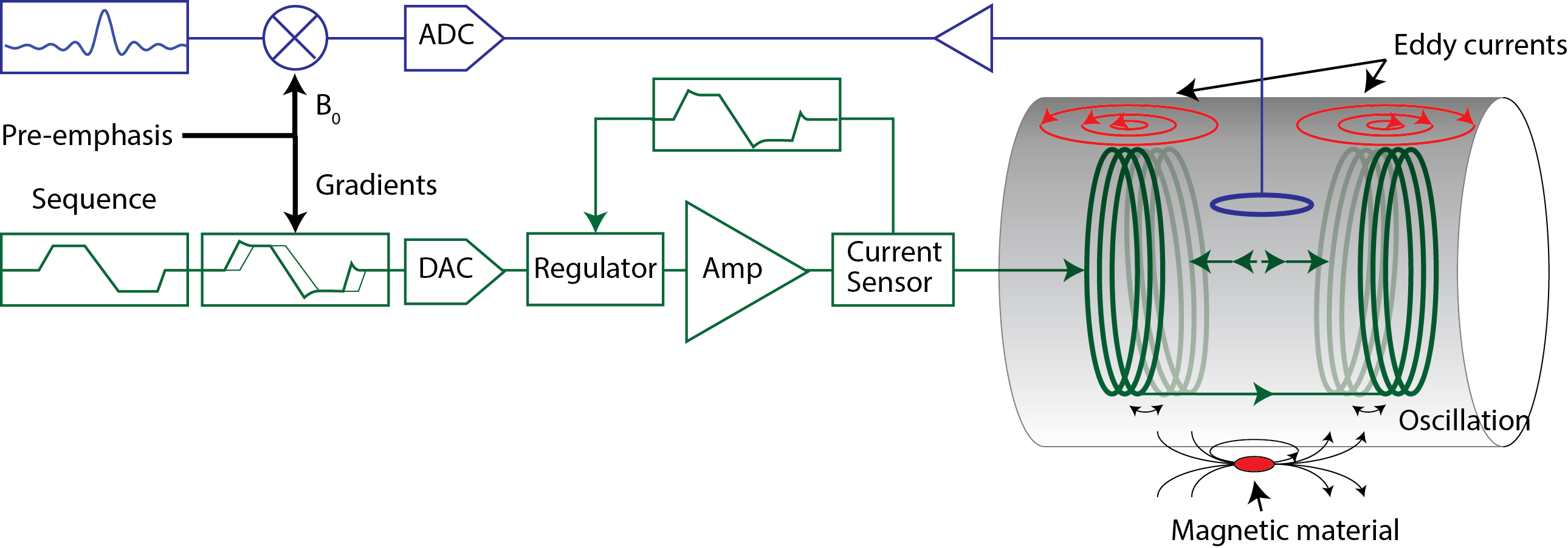
The spatio-temporal dynamics of the magnetic field inside the scanner generates and encodes the NMR signals. In order to interpret and reconstruct images from the acquired raw signals the exact evolution of the magnetic field inside the scanner has to be accurately known. But the employed hardware cannot natively provide the accuracy in the field dynamics that is ideally required spatially and temporally. Spatially, the applicable equations of magnetostatics set limits on realizable field patterns. This leads to deviations of the field pattern generated by a gradient or shim coil from the targeted ideal distribution. A gradient coil would ideally produce a spatially linearly increasing field strength along a given axis. In reality there will be a spatial non-linearity of the field but the resulting image distortions can mostly be handled in post-processing by unwarping the images to remove the geometrical distortions [1]. Realizing the desired temporal evolution of the magnetic field in the scanner is more complex and furthermore subject to very tight tolerances. Stray induction into conductive surfaces, mechanical interactions and externally induced fields cause delays, distortions and fluctuations that heavily impair the resulting image quality. Deviations from the intended field evolution corrupt the acquisition in various ways; errors in the k-space trajectory of the read-out cause ghosting, warping and shading in the reconstructed images. Equally unwanted field transients affect the slice selection by exciting incorrect volumes leading to inconsistent data sets, loss of steady-state conditions or signal strength. Furthermore, currently developed advanced acquisition methods heavily push the need for accuracy of the sequence execution for speeding up the acquisition, deducing quantitative information or by requiring a high consistency between several acquisitions for later data fusion. Obviously deriving quantitative information requires a high degree of fidelity from the system but equally highly efficient encoding schemes turn out to be more susceptible to errors in the underlying encoding. For example EPI, UTE and spiral acquisitions are very susceptible to minute delays in the gradient encoding while magnitude images from normally employed Cartesian single line spin-warp read-outs are very robust against gradient delays. Similarly, fast sequences react very sensitive to steady-state violations due to their long echo-trains. Finally, the trend towards higher field strength sets even higher needs for stronger and faster switching gradients in order to provide on the one hand robustness against susceptibility artefacts by fast high-bandwidth read-outs and on the other to turn the increased baseline SNR into increased speed and resolution. In order to obtain the required accuracy in the field evolution, MRI scanners require therefore very accurate compensation and correction schemes in order to overcome the remnant shortcomings of the employed hardware. The basic principle behind this approach is that calibration, compensation and correction schemes can turn the precision and accuracy achieved in measurements of the magnetic field evolution into an enhanced fidelity of the acquisition and reconstruction. This in turn implies that the accuracy by which the field dynamics can be measured sets the ultimate boundary for the achievable requirements set by the experiments. To achieve this, three basic types of schemes are employed: · Feedforward or pre-emphasis corrections pre-distort the requested waveform sent to the input based on a system characterization such that the output fits the demand best. · Feedback approaches measure the deviations of the observable concurrently at the output of the system and correct the input in real-time to compensate for the deviations. · Post-correction schemes correct the value of the obtained measurement in the acquired data for the effect of known deviations present during the experiment. Figure 1 depicts the application of the three approaches on the example of a typical gradient chain. The main advantage of feedforward and feedback approaches is that they improve the fidelity of the physical execution of the experiment. The experiment can therefore be executed under almost ideal conditions. This is important because not all deviations can be post-corrected or inflict penalties in the conditioning or numerical complexity of the reconstruction problem. Generally, the effect must be encoded in the acquired data in order to be post-corrected out of the obtained data. For example an accurate execution of slice selection gradients is required in order to provide signal from the correct slice location, keep steady state conditions and avoid signal loss by through-slice dephasing all of which can typically not be post-corrected on the acquired data. For post-correcting errors of the read-out trajectory it has to be ensured that the signal is sufficiently encoded in order to render the reconstruction problem well-conditioned. There is however a bigger leeway since some of the encoding can be deferred to parallel imaging schemes. Finally, there are classes of acquisition schemes that encode all properties of the spin system such as stochastic resonance approaches [2] and MR fingerprinting [3]. In these cases, the acquisition can be post-corrected even from heavily distorted sequence executions as long as the randomization criteria and the bandwidth coverage remain fulfilled. However, it is then required to encode the entire scope of parameters, which might come with an overhead in the acquisition at least if some of the fitted values are not used in the end. The major downside of feedforward and feedback approaches is that they require additional driving power to play out the compensating waveform. This overhead has to be accounted for and limits the maximum available slew rates and amplitudes. Furthermore, feedforward approaches critically depend on the exact knowledge and stability of the system behavior to pre-distort the input waveform to the system since it needs to predict the field evolution based on the request. In contrast, feedback approaches are insensitive to small changes of the system but require an accurate concurrent measurement of the regulated entity with low delay and high bandwidth in order to keep the system stable. Magnetic field measurements are therefore typically not applied for feedback control of fast switching encoding gradients but can be well applied for correction of slow field drifts [4]. However, gradient amplifiers are equipped with current sensors regulating the output current. This feedback highly linearizes and equalizes the gradient chain with respect to the current in the leads. But the field evolution produced by the coil can deviate from that of the driving current in its terminals requiring additional correction in order to effectively ensure a precise image encoding. As mentioned above the major advantage of post-correction schemes is that they do not require additional driving power and do typically not interfere with the execution of the sequence but the conditioning of the reconstruction problem can worsen increasing noise in the result. In turn, post correction schemes can correct for field distortions where no actuation is available for compensation, e.g. higher spatial orders or outside the bandwidth gradient and shim channels in particular can operate in. Examples of such approaches that are regularly applied are correction of gradient induced B0 fluctuations which are typically implemented by shifting the frequency the acquired signals are demodulated with and/or the phase of the acquisition as for instance in EPI phase corrections [5]. Furthermore, the entire reconstruction can be based on predicted [6] or even concurrently monitored k-space trajectories [7] and even entirely monitored sequences [8] taking all field evolution into account. In summary, feedforward, feedback and post-processing corrections complete each other and are therefore almost exclusively applied in combination.

Encoding field generation and distortion effects

As shown in Fig. 1 the required gradient fields are generated by first converting the requested digital waveform into a low-power analogue signal, which is then sent to the gradient power amplifier stage. The gradient amplifier then drives the current through one gradient coil or a segment of it which produces the required magnetic field. Since the temporal evolution of the gradient and shim fields depend on the driven current waveform, very high fidelity waveforms have to be generated in the first place using high dynamic range waveform synthesizers. Due to the high power requirements, very power efficient topologies have to be employed in the gradient amplifier. Such topologies do not provide the needed accuracy and linearity. Therefore the gain stage is tightly controlled by a feedback mechanism. A current sensor, typically of a flux-gate type, dynamically measures the output of the amplifier and deviations are filtered and fed back to the input. This linearizes the amplifier over a large dynamic range and stabilizes it against various sources of drifts in the gain stage. Furthermore, the feedback renders the driven current independent of the load impedance at the output. This effectively compensates for the effect of the coil inductance and resistance within the feedback bandwidth. As a consequence the current driven through the terminals of the coils correspond very precisely to the requested waveform. By this feedback the field evolution in the coil is controlled to the degree the field inside the coil depends on the current through the terminal of the coil. There are however effects that let the field generated by the coil deviate from the current running through the terminals of the coil. Primarily current paths driven by induction caused by gradient switching do not run through the terminals and produce additional field. By Lenz’s law, these currents oppose the slewing of the field in the coil and therefore introduce a delay and slows down the ramping of the field. Furthermore, the field pattern is distorted from the field of these additional current paths. Currents induced in other gradient or shim coils produce a secondary field with predominantly the spatial pattern of the coupled channel and appear like an unwanted activation of that channel. These couplings to other gradient or shim channels are therefore called cross terms. However, ramping a magnetic field in bulk conductors causes locally flowing electric currents, the so called eddy currents. The quasi-stationary field ($$$B$$$) generated by impressed and induced currents ($$$J$$$) in conductive materials ($$$\sigma, \mu$$$) is governed by a diffusion equation: $$\sigma \mu \frac{\partial B}{\partial t}= \nabla^2 B=-\nabla \times J.$$ The equation links the temporal dynamics with the material properties and its geometry which shows that the eddy current effects and lifetime scale with the conductance of the material and its size. The larger the current path and the higher the bulk conductivity the longer the energy can be stored in the eddy and consequently the longer its time constant. Although, MRI scanners and the components present in the bore are designed to exhibit minimal contiguous conductor surfaces, eddies in the conductors of gradient coils, RF coils , RF screens, cryostat walls and cold structures critically distort the field evolution and have orders of magnitude different time scales and intensities. Eddies that produce the same field pattern as the generating coil cause a delay and low passing of the gradient pulses. Eddies that produce other field patterns by their current paths cause apparent cross-terms. In addition to induction of additional currents, the current carrying conductors are subject to strong Lorentz’s forces. Thereby the coils are deformed and consequently change their field pattern and efficiency. This is prominently visible at frequencies of mechanical resonances of the gradient coil former. If such a resonance is excited by the requested waveform the coil mechanically oscillates and produces and oscillatory field response. Such electromechanical oscillations can have very long decay times (several 10 to 100 ms) and occur typically above 1 kHz. Furthermore, the frequency and quality factor of the mechanical resonances are found to be highly dependent on the temperature of the gradient and shim coil due to the temperature coefficients of the mechanical properties of the employed formers. However, besides their temperature dependence the above mentioned effects are typically governed by linear equations. Although the field response of the coil is temporally and spatially distorted the output remains a linear response of the current driven through the coil. But besides inductive and mechanical couplings also thermal effects can cause field distortions. Particularly thermal coupling from the gradient coil to passive shim irons can cause field drifts. This coupling is not a linear response to the driven sequence. The heating induced in the gradient coils depends on the root-mean-square current but also on the driven slews but equally on the system cooling and ambient factors. These effects are therefore very hard to characterize up-front and are typically tackled by run-time measurements for instance by re-determining the NMR center frequency of the sample or by use of external references [9] for monitoring the field evolution. Finally, there can be induced field dynamics in the scanner which is not driven by the scanner at all. Such fields can originate from close by installations such as elevators, moving cars, power lines, train tracks etc. But also the subject can induce field variations by breathing or limb motion [10] which moves susceptible material in the bore. Correspondingly, these effects cannot be calibrated nor predicted and need to be either suppressed or post-corrected based on concurrent measurements of the field evolution [11].

Measurements

Irrespective if feedforward, feedback or post-correction schemes are applied the field evolution has to be measured in the first place. Based on these measurements the system can then be characterized in order to be calibrated and corrected. Ideally, the magnetic field evolution in the scanner is captured with high temporal and spectral resolution and a spatial resolution that allows separating the different involved cross terms. Basic calibration schemes however have only to determine the delay of the individual channels and the most important decay times of the involved eddy currents. The latter can be very efficiently implemented using NMR based measurements on phantoms [12-15]. Thereby simple blip encodings can be employed to study the temporal alignment and phase evolution of the echoes representing the individual delays of the gradients. Even entire k-space trajectories and higher spatial orders can be acquired using spatial-spectrally encoding the phase evolution driven by the trajectory [16]. The main advantage of these methods is that they do not require additional hardware besides the phantom. However, for resolving spatial-spectral field dynamics the methods have to acquire several shots with very high consistently and the additionally required additional gradient lobes must not affect the measurement. Therefore, the MRI system has to be stable and repeatable over all these shots and fluctuations and drifts can often not be quantified and hamper the calibration. Furthermore, they require a very well shimmed setup to characterize long term effects and also the gradient system has to operate accurately enough to perform correct excitations and encodings of the trajectory. This poses a certain bootstrapping problem in particular at installation of the scanner. Typically this is circumvented by first shimming the magnet using an external field mapping device. Alternatively external field measurement devices can be employed to measure the gradient dynamics. A comparably simple method is based on pick-up loops which sensitize the induction caused by the gradient ramping [17]. While they can very well detect channel delays, they often do not deliver enough sensitivity to measure long term eddy currents, field drifts or to map an entire k-space trajectory. This is because they measure the induction and in order to determine the phase accrual induced to the spins their signal has to temporally integrated twice, which has very unfavorable noise propagation properties. Recently NMR based field probe systems [7, 11, 18] are increasingly used. The NMR signal offers a very high sensitivity to detect the relevant magnetic field component as well as its time integral even with high bandwidth. By employing an array of such sensors the spatial-temporal field evolution can be measured in a single shot and even during the actual experiment. Therefore, transient effects, drifts and even subject induced effects can be acquired. Furthermore, the actual field evolution during the experiment can be captured and applied in the post processing step. On the downside the method requires additional involved hardware.

Synchronization

When interpreting the calibration data acquired with the MR scanner as well as with external devices the problem of synchronicity has to be concerned. While the NMR sequence is acting on the spins and the spins produce their signal in the physical time frame, the time frames the MRI scanner’s sequence programs are operating in is typically a different digital time raster (see Fig. 2). Since the different subsystems such as RF transmit, receive, gradient and shim chains exhibit different delays relative to the physical time frame there can be discrepancies between the different time rasters. A particular problem is that the delay of the RF chains can be critically dependent on the loading condition of the RF coils. Furthermore, the physical time frame is only observable via the receive chain. Therefore the system is typically calibrated to a roughly compensated discrete receiver time raster. In turn, a system which has an apparently synchronized gradient and receiver system can still exhibit systematic delays between the transmitter and the gradient chain as well as the receiver.

Gradient system characterization

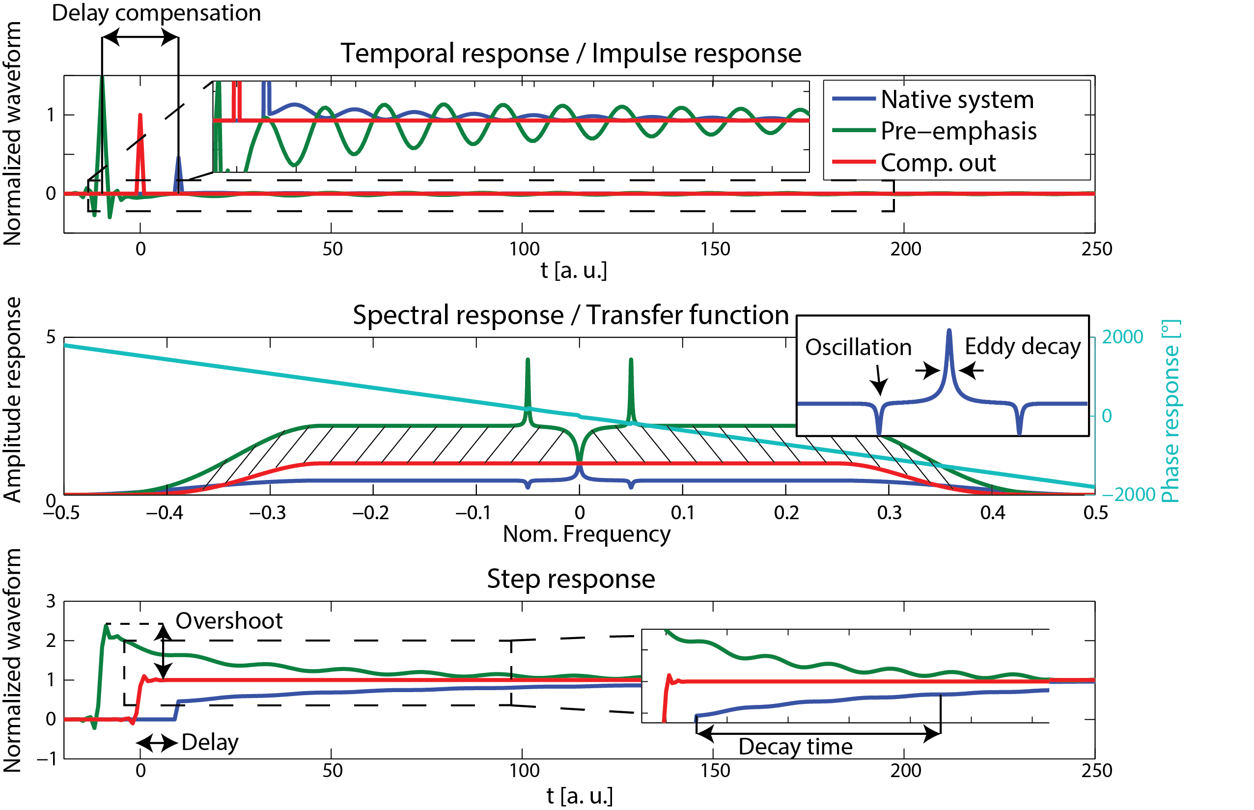
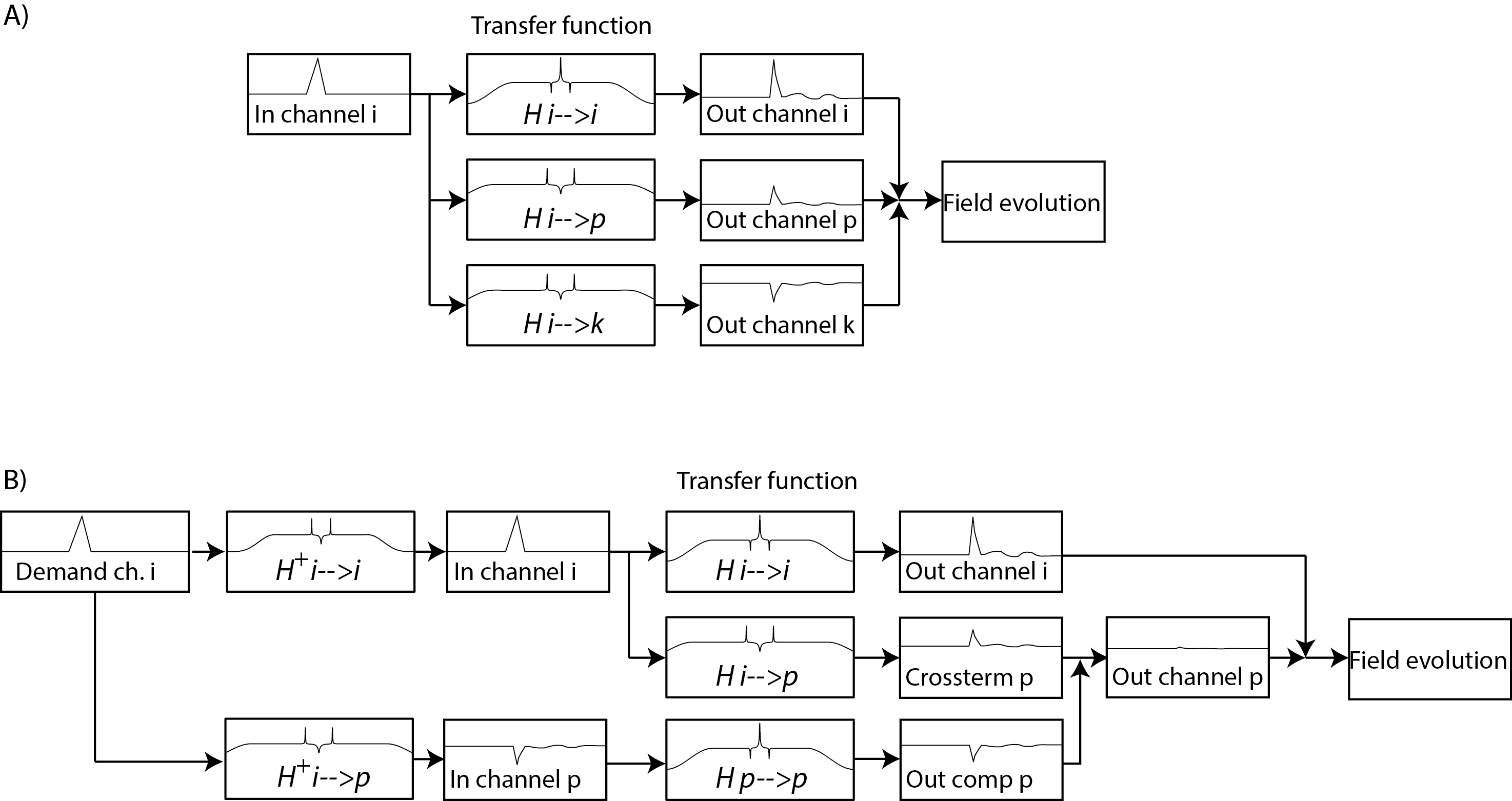
The goal of a system characterization is to predict the output of the system dependent on its given inputs. This knowledge can then be used for calibration, feedback adjustments, post-correction and sequence optimization. Fields induced by sources not under control of the scanner or that are not dependent on accessible variables cannot be considered for a calibration and represent therefore a constant source of potential confounders of the calibrated system’s output but also for the calibration procedure itself. However for calibration purposes the MRI system has to be considered as time invariant and it remains to other means that other confounders are minimal. Additionally, the gradient and shim systems can be to a very large degree considered as linear systems, i.e. the field output is considered linearly dependent on the demand sent to the system [19]. Ensuring this linearity however is a critical effort in the hardware design and is ensured by very involved feedback driving circuits as mentioned above. As a consequence of the linearity and time invariance, the field output ($$$B(r,t) = \mathcal{F}^{-1}(b(r,\omega))$$$) is given as convolution of the demanded waveform ($$$ D(t) = \mathcal{F}^{-1}(d(\omega))$$$) and the impulse response function ($$$IR(r,t) = \mathcal{F}^{-1}(H(r,\omega))$$$) of the system: $$B(r,t) = D(t) \otimes IR(r,t),$$ or analogously in frequency domain: $$b(r,\omega) = d(\omega) \cdot H(r,\omega).$$ The calibration sequences characterizing the system have therefore to provide the data basis to determine the transfer function within the required bandwidth. This is achieved by recording the field output for a set of known inputs which cover the required frequency span. The transfer function is then found by a deconvolution of the output with the input signal: $$H(r,\omega) = \frac {b(r,\omega)}{d(\omega)}.$$ In principle various test functions ($$$d(\omega)$$$ can be employed as input such as blips or sweeps as long as the system is not driven to substantial non-linearity arising from amplitude or slew-rate limitations. Figure 3 shows an example for the response of a y gradient coil to a trapezoidal blip. The impulse response and equally the transfer functions contain all the information on delay, eddy currents oscillations etc. as depicted in Fig. 4. As seen, the delay causes the impulse response function of the native system to peak after the demand and the transfer function exhibits a corresponding phase gradient. The eddy current terms low pass the response which causes the transfer function to be below the requested amplitude at higher frequencies. Correspondingly, the calculated step response creeps slowly to the targeted value. Finally, the oscillations visible in the transfer function as clear dips cause the field fluctuate around the target value ones excited by a step in the targeted field. In order to characterize the spatial behavior of the dynamic fields it is recommendable to decompose the spatial degrees of freedom into a set of spatial basis functions $$$B_i(r), i = 0, …n$$$: $$B(r,t)=\sum_{i=0…n} B_i(r)\cdot J_i(t),$$ $$b(r,t)=\sum_{i=0…n}B_i(r)\cdot j_i(\omega).$$ The components $$$J_i(t)=\mathcal{F}^{-1}(j_i(\omega))$$$ represent the time evolution of the field pattern. Choosing the spatial field pattern of the individual gradient and shim coils as such a spatial basis is often very insightful since the coupling terms are directly visible in the activation of the corresponding components ($$$J_i(t)$$$). Consequently, the impulse responses and the transfer function can be decomposed in the same spatial basis and with respect to every possible input waveform ($$$D_p(t)$$$) which yields: $$B(r,t) = \sum_{i=0…n} B_i(r) \cdot J_i(t) = \sum_{i=0…n, p=0…n} B_i(r) D_p(t) \otimes IR_{i,p}(t)$$, $$b(r,t)= \sum_{i=0…n, p=0…n} B_i(r) d_p(\omega) \cdot H_{i,p}(\omega).$$ The system’s response is then characterized by a matrix of transfer/response functions. The response of the channel to itself is characterized in the $$$ IR_{Iii}(t)$$$ functions, the cross-term couplings are represented in the off-diagonal functions.

Feedforward compensation

The basic idea of feedforward compensations is to pre-distort the requested waveform such that the field evolution will fit the request within the targeted bandwidth. For instance a delay can be compensated by playing out the waveform earlier such that it will arrive in time. Each frequency component is scaled and phased based on its characterized response such that it will be equalized at the output, which is called pre-emphasis. Since eddy currents and other band-limiting effects lower the efficiency of the gradient system at higher frequency, these components have to be scaled up in the demand sent to the amplifier, which results in a required overdrive in the pre-distorted waveform. The amplifier has consequently to produce higher output voltages or currents in order to speed up the ramping of the fields and to suppress cross terms. This in turn limits effective slewing and peak values of fields that can be requested when designing the not pre-emphasized waveform. Therefore it is important to limit the targeted response of each channel to the minimum required bandwidth by using a windowing function ($$$W(\omega)$$$) attenuating the request for high frequency components. Then the pre-distorted waveform ($$$D^C(t) = \mathcal{F}^{-1}(d^C(\omega)$$$) can be calculated by a deconvolution operation as also depicted in Fig. 4: $$d^C(\omega) = \frac {d(\omega) \cdot W(\omega)}{H(\omega)} = d(\omega) \cdot H^+(\omega),$$ $$D^C(t) = D(t) \otimes IR^+(t),$$ where $$$H^+(\omega)=\frac{W(\omega)}{H(\omega)}$$$, and $$$IR^+(t) = \mathcal{F}^{-1} (H^+)$$$. Analogously cross-terms can be suppressed by inverting the transfer function matrix for each frequency (see Fig. 5): $$H^+(\omega) _{i,p} = W(\omega) \left ( H(\omega)^ {-1} \right )_{i,p} \forall \omega.$$ Also here other channels have to allocate overhead power in order to compensate for the coupling. Therefore the inversion of the transfer matrix has to be carefully regularized by use of an appropriate pseudo-inverse ensuring a well-conditioned inverse at every frequency. In many cases the calculation of the pre-distorted waveforms is simplified and numerically optimized by translation to time domain filters. Due to the involved long integration times this is often implement as infinite impulse response filters. For this, the impulse response of the system has to be decomposed into the individual elements of the filter. A further major consideration of feed-forward approaches is that the convolution kernel obtained for the pre-emphasis is not causal. This means that it has to be known in advance what waveform will be required in order to send out the signal in time. This is for typical sequence execution no problem since the waveforms are known well ahead of time. However, it can become a consideration limiting the reaction time in real-time applications for triggering, prospective motion correction or field feedback.

Feedback compensation

Feedback approaches offer the advantage that the behavior of the native system can vary to a certain degree maintaining the overall output if the measurement of the feedback variable is not affected, the system remains stable and does not overshoot out of the regulation. However, in order keep the feedback stable, the output value has to be measured with very low delay compared to the bandwidth the feedback is supposed to operate in. Therefore, feedback of fast gradient waveforms is typically only applied to the output current of the amplifier, which can be measured very fast and with high accuracy. This linearizes the gradient amplifier and compensates drifts and gain changes of its output stage. Furthermore, the low-pass frequency response of the gradient coil with regards to its input current is largely compensated by this feedback circuit. Additionally, the feedback loop of the amplifier produces a very high impedance at its output which largely hinders net currents to flow due to induction from other channels. However, as mentioned above the controlled value is the current present at the terminals of the amplifier, whose dynamics can differ from that of the field inside the coil. Nevertheless, low frequency drifts can be well compensated using either short frequency navigator acquisitions or independent field monitoring devices [4]. Since many of these drift effects are not captured by the feedforward calibration of the system, the feedforward and feedback approaches complement each other very well.

Post-correction

Post-correction of the acquired data compensating for individual effects of the gradient chain distortion is widely implemented at different stages of the signal processing on current MRI scanners. E.g. the NMR frequency shifts induced cross-terms to the uniform field for instance caused by long lived eddy currents as generated by diffusion sensitizing gradients is demodulated out of the acquired data by the eddy current correction system. The phase inconsistency of odd- and even-echo tops is typically corrected for in EPI scans [5] by shifting the phase of the acquired signals. Gradient chain delays are often compensated for in reconstruction UTE sequences etc. However, in principle the full system characterization can be employed to predict the field evolution during a scan in order to obtain the k-space trajectory of given scan [6]. Furthermore, concurrent field measurements can be employed [7, 20, 21] to obtain the effective gradient encoding of a scan as it was present during the acquisition. These measurements then not only include the predictable field evolution based on the demanded sequence but also externally, temperature and subject induced effects which can then be handled by the reconstruction.

Acknowledgements

No acknowledgement found.