Synopsis

This presentation will provide an overview of the main gradient echo based (gradient spoiled, RF spoiled and balanced steady state free precession) and conventional/fast spin echo based pulse sequences and will illustrate some methods by which their behaviour can be simulated.

Introduction

The behaviour of the magnetisation in a pulse sequence is described by the Bloch equations (1) and a number of methods have been utilised to simulate the behaviour of spins in an imaging sequence such as the matrix formalism (2), the use of extended phase graphs (EPG) (3, 4), pictorial representations (5) and analytical descriptions (6, 7). The examples given in this lecture are based upon code from Brian Hargreaves' Bloch equation simulations (http://mrsrl.stanford.edu/~brian/bloch/), Matthias Weigel's EPG simulations (http://epg.matthias-weigel.net/) and a Matlab implementation of the C program given in Klaus Scheffler's article (5).

Gradient Echo (GE)

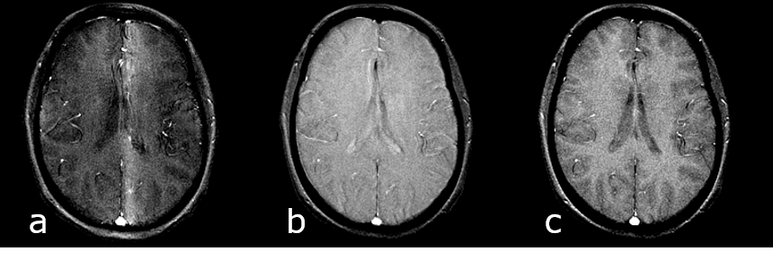
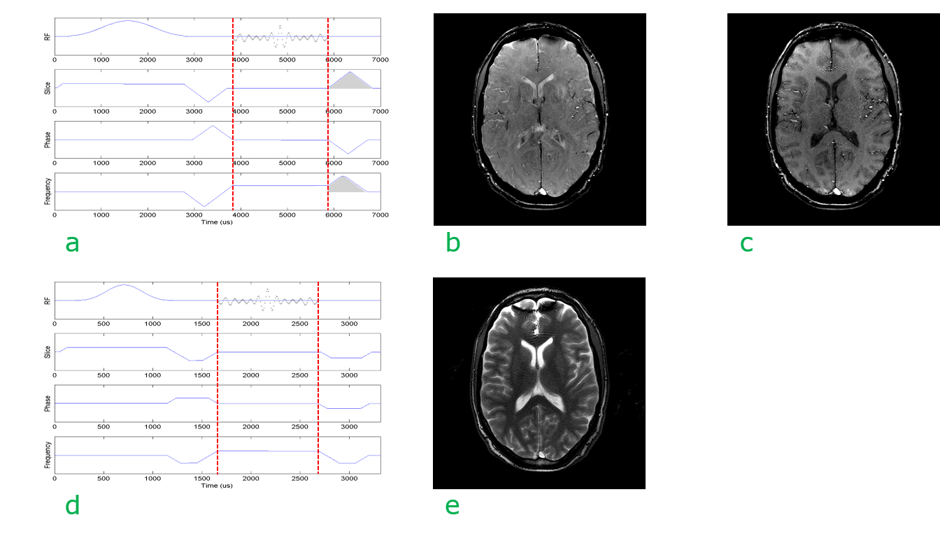
A gradient echo sequence comprises a train of equally spaced radiofrequency (RF) excitation pulses and the necessary gradients to perform slice selection, phase encoding and frequency encoding. The echo signal is formed by the application of a negative dephasing gradient followed by the frequency encoding gradient. The minimum echo time (TE) is dependent upon the RF pulse duration, receiver bandwidth and available gradient performance. Usually the time between excitation pulses (TR) is short and the transverse magnetisation has not had time to fully dephase. Since the phase encoding gradient is the only gradient that changes between TRs the transverse magnetisation will have a position-dependent distribution of resonant offset phase angles across the slice, which will affect the signal created by the subsequent RF pulse. As a result, bands of varying signal intensity, known as "FLASH-bands" may appear degrading the image quality (Figure 1a). The three main gradient echo sequences differ in how they deal with this residual transverse magnetisation: a) the gradient spoiled sequence averages the resonant offset phase distribution across a voxel (Figure 1b), b) the radiofrequency (RF) spoiled sequence eliminates the transverse magnetisation (Figure 1c) whilst c) the balanced steady state free precession (bSSFP) sequence rephases the phase distribution. Example pulse sequence diagrams and images are shown in Figure 2.

Gradient Spoiling

The gradient spoiled sequence has additional gradients applied after data acquisition on the slice select and frequency encoding axes (Figure 2a) that averages the resonant offset phase distribution across a voxel. The phase encoding gradient is "rewound" so that the dephasing gradients are constant across TRs. Figure 2b shows an axial head image obtained using a gradient spoiled sequence.

RF Spoiling

The gradients are the same for both the gradient and RF spoiled sequences (Figure 2a), but the phase of the RF excitation pulse is incremented, usually quadratically, on each excitation.

$$ϕ_j = \frac{1}{2} ϕ_0 (j^2+j+1),j=0,1,2,…$$

There are certain “magic numbers”, e.g. φ₀=117°, for the phase increment that can produce excellent spoiling across a range of T₁, T₂ and excitation flip angles (8) and is equal to the steady-state transverse magnetisation for a perfectly spoiled sequence given by the Ernst equation

$$M_{ss}=M_0 (1-exp(-TR/T_1 ))/(1-cos(α) exp(-TR/T_1 ) ) \cdot sin(α)$$

Balanced Steady State Free Precession (bSSFP)

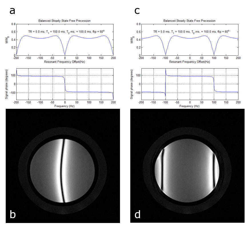
The bSSFP sequence (Figure 2d) has all gradients balanced, i.e. there is zero net gradient area on each axis over a TR period. Any resonant offset phase errors will therefore not be averaged. This means that the signal response is dependent upon the phase offset. Figure 3 shows a simulation of the signal behaviour as a function of resonant offset phase angle for two excitation schemes. In Fig 3a and 3b there is no phase offset applied between subsequent RF pulses. In Figure 3c and 3d the phase of the RF excitation is alternated between 0 and 180°. In this example a large left-right shim offset of 14.7Hz/cm was applied. The resonant offset is given by θ=2π·Δf·TR and the signal nulls or bands appear at θ=±π, or when Δf=±1/2·TR. In this case the TR was 5ms resulting in bands appearing at ±100Hz. Figure 2e shows the image obtained using a bSSFP sequence. Note an off-resonance band can be seen anteriorly. The steady state signal for a bSSFP sequence, assuming that TR«T₁,T₂ is given by

$$M_{ss}=M_0 \frac {sin(α)} {(1+cos(α)+(1-cos(α) ) \cdot \frac{T_1}{T_2}}$$

The optimal flip angle is given by

$$cos(α)=\frac{\frac{T_1}{T_2} -1}{\frac{T_1}{T_2} +1}$$

which results in a steady state signal of

$$M_{ss}=\frac{1}{2} M_0 \sqrt{\frac{T_2}{T_1}}$$

Hence tissues with a high T₂/T₁ ratio, e.g. fluids, will exhibit a high signal.

Spin Echo (SE) and Fast/Turbo Spin Echo (FSE/TSE)

Spin Echo

Spin echo (SE) is a basic pulse sequence comprising typically of a 90° and a 180° RF pulse. The initial 90° excitation pulse tips the longitudinal magnetisation into the transverse plane where it naturally dephases due to T₂^* relaxation processes. After a time τ the 180° refocusing pulse is applied which rotates the transverse magnetisation 180° about the axis along which the pulse is applied. This rotation effectively inverts the phase of the magnetisation so that it now naturally rephases, coming fully back into phase, and forming what is known as a spin echo, after a further time period τ. The time between the initial 90° excitation pulse and the centre of the echo is known as the echo time (TE) and is equal to 2τ. The effect of the refocusing pulse is to eliminate the effect of any static magnetic field non-uniformities from the T₂^* signal therefore leaving any signal differences due to irreversible T₂ interactions. The magnetisation will then recover along the z-direction due to T₁ relaxation until the application of the next 90° pulse. The time between repeat applications of the 90° pulse is the repetition time (TR). The signal is given by

$$M=M_0 (1-exp(-TR/T_1 )\cdot exp(-TE/T_2)$$

Fast/Turbo Spin Echo

Proton density or T2-weighted spin echo sequences are particularly slow since they require a long TR in order for there to be appreciable longitudinal magnetisation recovery before the next excitation pulse. Although the acquisition of other slices can be interleaved within the TR period the sequence is still not particularly efficient. Fast, or turbo, spin echo (FSE/TSE) was developed as a method for reducing the overall acquisition time (9). The basic principle is to use a Carr-Purcell-Meiboom-Gill (CPMG) multi-echo spin echo acquisition, where the transverse magnetisation is repeatedly refocused by the application of a train of refocusing pulses forming multiple spin echoes each at correspondingly increasing TEs. If each echo is individually phase encoded, then they can be used in the same image k-space resulting in a shorter acquisition time. It is necessary to arrange the amplitudes of the phase encoding gradients so that the echo nearest the desired TE - known as the effective echo time (TEeff), has the lowest amplitude phase encoding gradient, i.e. that echoes’ data will be nearest the centre of k-space. The interval between refocusing pulses is known as the Echo Spacing (ESP) and the number of refocusing pulses per TR is known as the Echo Train Length (ETL). Since multiple echoes are acquired per TR there is also a filtering effect due to the T₂ decay of the echo amplitudes over the ETL. The T₂ decay results in a broad point spread function which has the effect of blurring the images. A limitation of FSE is the relatively large power deposition associated with long echo trains. A common solution to this problem is to use reduced flip angle refocusing pulses that substantially reduce the power with only a minor impact on the signal-to-noise ratio (SNR). The use of refocusing pulses <180° do, however, give rise to a number of coherence pathways which lead to the creation of a so-called pseudo-steady-state (PSS) (10). These coherence pathways can be most easily studied using the EPG method in which the magnetisation is described as sub-states which are defined as groups of spins with different M_x, M_y and M_z (3). Figure 4 shows a hand-drawn EPG for an initial excitation pulse followed by three refocusing pulses . The essential feature of the phase graph concept is that after an RF pulse has been applied the magnetisation behaves as a composition of three parts a) dephasing transverse magnetisation, b) rephasing transverse magnetisation and c) longitudinal magnetisation (4). The dephased magnetisation after the excitation pulse is labelled F₁. The first refocusing pulse will invert a component of the magnetisation, creating the F-1 sub-state and will also produce z-magnetisation represented by Z₁ and its complex conjugate Z_-1. Since the phase information does not evolve with time these longitudinal sub-states are represented as horizontal (red) lines. The dephasing of F₁ gives rise to F₂, whilst rephasing of F_-1 causes the formation of a echo (F₀) shown by the pink circle. Further time evolution creates higher order sub-states which contribute to the amplitude of each echo. The evolutions of transverse sub-states from larger numbers of pulses are usually displayed as shown in Figure 5.

Summary

Acknowledgements

References

1. Bloch F. Nuclear induction. Phys Rev 1946; 70:460-474.

2. Jaynes E. Matrix treatment of nuclear induction. Phys Rev 1955; 98:1099-1105.

3. Hennig J. Multiecho imaging sequences with low refocusing flip angles. J Magn Reson 1988; 78:397-407.

4. Weigel M. Extended phase graphs: dephasing, RF pulses, and echoes - pure and simple. J Magn Reson Imaging 2015; 41:266-295.

5. Scheffler K. A pictorial description of steady-states in rapid magnetic resonance imaging. Concepts in Magn. Res. 1999; 11:291-304.

6. Sobol WT, Gauntt DM. On the stationary states in gradient echo imaging. J Magn Reson Imaging 1996; 6:384-398.

7. Hanicke W, Vogel HU. An analytical solution for the SSFP signal in MRI. Magn Reson Med 2003; 49:771-775.

8. Zur Y, Wood ML, Neuringer LJ. Spoiling of transverse magnetization in steady-state sequences. Magn Reson Med 1991; 21:251-263.

9. Hennig J, Nauerth A, Friedburg H. RARE imaging: a fast imaging method for clinical MR. Magn Reson Med 1986; 3:823-833.

10. Alsop DC. The sensitivity of low flip angle RARE imaging. Magn Reson Med 1997; 37:176-184.

11. Busse RF, Riederer SJ. Steady-state preparation for spoiled gradient echo imaging. Magn Reson Med 2001; 45:653-661.

12. Le Roux P. Simplified model and stabilization of SSFP sequences. J Magn Reson 2003; 163:23-37.

13. Hennig J, Scheffler K. Easy improvement of signal-to-noise in RARE-sequences with low refocusing flip angles. Rapid acquisition with relaxation enhancement. Magn Reson Med 2000; 44:983-985.

14. Hennig J, Weigel M, Scheffler K. Calculation of flip angles for echo trains with predefined amplitudes with the extended phase graph (EPG)-algorithm: principles and applications to hyperecho and TRAPS sequences. Magn Reson Med 2004; 51:68-80.

15. Worters PW, Hargreaves BA. Balanced SSFP transient imaging using variable flip angles for a predefined signal profile. Magn Reson Med 2010; 64:1404-1412.

16. Busse RF. Reduced RF power without blurring: correcting for modulation of refocusing flip angle in FSE sequences. Magn Reson Med 2004; 51:1031-1037.

17. Ma D, Gulani, V, Seiberlich, N et al. Magnetic resonance fingerprinting. Nature 2013;495:187-192