Synopsis

The NMR (Nuclear Magnetic Resonance) signal can be described classically by considering the motion of the net magnetisation (the vector sum of magnetic moments of individual nuclei). By considering individual isochromats – i.e. subsets of the spins that are behaving identically– we can visualise how the received signal will decay away due to T₁, T₂ and T₂^* relaxation. By additionally considering the effects of magnetic field gradients, we can determine the spatial location of the signal, producing images. All these effects can be described by the Bloch equations, which give complete classical description of the behaviour of magnetisation.

Highlights

• The production of an NMR (Nuclear Magnetic Resonance) signal can be described classically by considering motion (and in particular precession) of the net magnetisation (the vector sum of magnetic moments produced by individual nuclei).
• By considering how precession is affected by the application of linear magnetic field gradients, we can envisage ways to spatially localise the signal, leading to MRI (Magnetic Resonance Imaging).
• By considering individual isochromats – i.e. subsets of the spins that are behaving identically in terms of their orientation and precession – we can also visualise how the received signal will decay away. This decay (described mathematically in terms of the relaxation times T₁ and T₂ (and T₂*) differs between tissues, allowing us to sensitize our images to particular pathologies.
• The Bloch equations give complete classical description of the behaviour of magnetisation under influence of an applied field, and of relaxation.

Target Audience

Objectives

- Following this lecture, audience members should be able to:

- Discuss the basic concepts of the classical description of Nuclear Magnetic Resonance (NMR), in terms of:

• Magnetic moments
• Isochromats
• Net magnetisation
• Precession
• Nutation

- Understand how the use of magnetic field gradients allow us to extend the concepts of NMR to Magnetic Resonance Imaging (MRI).

- Understand how relaxation can be described is the classical model, and how relaxation times affect image contrast.

- Be aware of the Bloch Equations, and their use to calculate the evolution of the net magnetisation during an NMR/MRI experiment.

Purpose

From the Quantum Mechanical to the Classical Description

Background

Nuclear Magnetic Resonance (NMR) is a technique - first reported (independently) in 1946, by Purcell, Pound and Torrey[1] and Bloch, Hansen and Packard[2] - based on the resonance (i.e. matching) effect between properties of (some) nuclei and a magnetic field. In medical fields it is common to also hear the terms MRS (Magnetic Resonance Spectroscopy) and MRI (Magnetic Resonance Imaging), both of which utilize the same underlying NMR phenomenon. While a full description of NMR requires a quantum mechanical approach, many aspects of NMR (and thus MRI/MRS) can be explained in classical terms, by considering the nuclei as simple magnetic dipoles with a magnetic moment (μ). Quantum mechanics tells us that in a magnetic field B₀, nuclei with an angular momentum I will have 2I+1 energy levels (labelled by a value m, running from -I to +I). For “spin half” nuclei (I = ½) such as hydrogen, there are just two levels (m = +/- ½), which are often referred to as ‘spin up’ (m = -½) and ‘spin down’ (m = +½), which can be thought of as representing “spins” which are either “aligned with” or “aligned against” the magnetic field. The energy levels differ by:

$$\triangle E = \frac{\mu B_0}{I} = \gamma B_0 \frac{h }{2\pi}$$

where γ is the gyromagnetic ratio and h is Planck’s constant. The number in each energy level is governed by a Boltzmann distribution:

$$\frac{N_{up}}{N_{down}} = e^{- \frac{\triangle E }{kT}}$$

The difference in ‘up’ and ‘down’ spins, which is approximately 1 in 10⁶ at room temperature, is responsible for measured NMR signal.

Classical Description

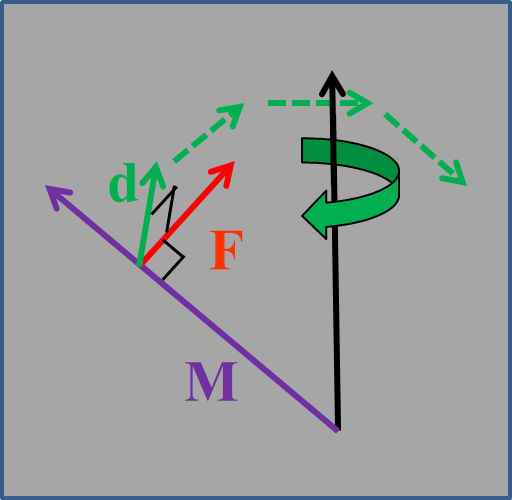
Following Farrah & Becker [3], "Our approach is to treat M as a measurable and easily pictured quantity and to avoid, in so far as possible, detailed discussion of quantization conditions". If we place tissue (or anything else containing suitable 'spin ½' nuclei) in a magnetic field it becomes magnetised, with a magnetic moment, M, aligned along the main magnetic field, B₀. Individual “spinning” nuclei behave like gyroscopes, and if disturbed, they react by moving in a direction d at right angles to both the applied (magnetic) force F and to their spin (along M) (Figure1). The spins precess around B₀ at the Larmor frequency, given (in radians s^-1) by:

$$\omega_0 = 2 \pi \nu_0 = \gamma B_0$$

We generally need to consider only the net magnetisation (i.e. the vector sum of the individual moments), which acts like a bar magnet (although we will sometimes also need to consider individual isochromats – i.e. subsets of the spins that are behaving identically in terms of their orientation and precession). The net magnetisation has magnetic moment given by $$$M_0 = \chi B_0$$$ where χ = susceptibility and B₀ is the applied magnetic field. An additional (small) internal field, caused by magnetisation itself, and equal in value to it, means total field is $$$B_{int} =B_0(1+ \chi)$$$. (This susceptibility effect can often be ignored, but will become important when discussing gradient echoes, echo-planar imaging and spectroscopy).

The Rotating Frame, Nutation Pulses and the Free Induction Decay

The Rotating Frame

So far we have viewed M in a static (laboratory) frame of reference. Any reference frame is equally valid, but it may be much easier to explain certain effects in one frame than another. (Describing the trajectory of a ball thrown inside a moving train is much easier in a frame of reference moving at the same speed as than train than it would be in terms of a viewer stood on the track side, for example). For NMR/MRI, easiest frame is one rotating with respect to the laboratory frame. If this frame is rotating in same direction as, but slightly slower than, the precessing magnetization, then in this frame the magnetization will appear to be precessing more slowly than in laboratory frame, and if we gradually increase speed of the rotating frame, the magnetization will eventually appear stationary, which make calculation of any further motion of the net magnetisation much easier. Since we have defined the precession frequency in terms of magnetic field however (through the Larmor Equation, $$$\omega_0 = \gamma B_0$$$), then if ω = 0 then B (in this frame) must be zero (!). Mathematically, the magnetization sees an effective field B_eff equal to the field in laboratory frame (i.e. B₀) minus an extra 'fictitious' field ω /γ:

$$ B_{eff} =B_0 - \frac {\omega}{\gamma}$$

When ω = ω₀ (i.e. when the rotation speed of the frame of reference is identical to the rate of precession of the spins), B_eff = 0, making our mathematical description consistent with the fact that the spins are no longer moving (relative to the rotating frame).

Nutation pulses

If we now (briefly) apply a field B₁, perpendicular to B₀ and rotating at ω₀, then in the rotating frame (also rotating at ω₀) B₁ will be stationary. B₁ is the only effective field in this frame, and M will therefore precesses about it, rotating away from z-axis towards xy-plane at an angular rate of $$$\omega_1 = \gamma B_1$$$ (the Larmor Equation again). When we turn off B₁, the magnetisation will have been rotated by a tip angle (or flip angle) given by $$$\theta = \omega_1 \tau = \gamma B_1 \tau$$$ where τ = duration of the pulse. A 90^o pulse has a duration of $$$\frac{\pi}{2\gamma B_1}$$$, while a 180^o pulse has a duration of $$$\frac{\pi}{\gamma B_1}$$$, etc, etc…

Resonance

Resonance is “The condition of a body when it is subjected to periodic disturbance of the same frequency as the natural frequency of the body or system” (Collins English Dictionary) - think of a wine glass 'ringing' - or “The condition of a system in which there is a sharp maximum probability for the absorption of electromagnetic radiation” (Ibid). Quantum mechanically, transitions between energy levels occur only when a photon of the correct energy is applied, while in the classical formalism magnetic moments (and therefore the net magnetisation) are only affected when a radio wave of a particular frequency is applied; in the static (laboratory) frame, nutation pulses correspond to magnetic fields varying at the resonant frequency, i.e. to radio frequency (RF) pulses.

Free Induction Decay

Faraday's Law tells us that a moving magnet will induce a current in a surrounding/nearby electrical conductor, and following a 90^o nutation pulse, the transverse magnetization (M_xy) constitutes such a moving magnet. A nearby coil can therefore detect a Free Induction Decay (FID) signal. (NB - M_z does not give a signal, as it is stationary with respect to the laboratory frame, and therefore the coil). The initial amplitude of the FID is proportional to the proton density (i.e. the concentration of the nuclei contributing to the signal), and the signal decays to zero with time constant T₂^* (see later).

Imaging

Field Gradients

By convention, the main magnetic field, B₀, is aligned with z (usually along the bore of the magnet); a field gradient along x, for example, means that the strength of the magnetic field (still itself aligned in z direction) varies with position along x.

$$B = B_0 + G_x x$$

The scanner hardware can create linear gradients in x, y, and z and, by applying gradients simultaneously on multiple axes, in any arbitrary, direction. To understand why this is useful, consider what happens when magnetic field, B, is not uniform over the object: If the field increases linearly with position, then resonant frequency must also increases linearly with position, which implies that we can use frequency to spatially encode the signal; by acquiring signals while gradients are applied in a number of direction, we can build up projections from which a complete image can be reconstructed. Early scanners used such a projection-reconstruction approach (which is similar to how a CT scanner works), but it turns out to be difficult to reconstruct artefact free images from projections, which has led to an alternative approach called spin warp imaging (which uses a phase encoding technique) becoming much more common. It is also technically difficult to measure a signal immediately after a 90^o pulse (and doing so doesn’t allow us to control the degree of signal decay due to T₂ or T₂^* (which we discuss below), so images are usually acquired using an echo based technique (also discussed below).

Spin Warp Imaging

Creating an image requires encoding of spatial positions in 3 dimensions. In 2D imaging, we first select a slice, and then perform spatial encoding in 2 directions, usually repeating the process for a number of slices, in order to cover the whole object. For 3D imaging, we may choose to select a “slab” (i.e. a single thick slice) from which we will collect signal, or may opt to collect signal from the whole object being imaged, but in either case will need to spatial encode the resulting signal in 3 directions. A full description of spatial encoding techniques commonly used is beyond the scope of this talk, but very briefly:

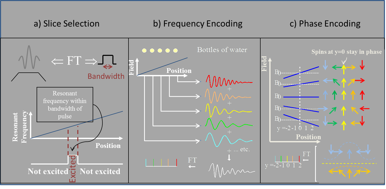
Slice selection: Slice (or slab) selection is achieved by using a shaped RF pulse in presence of a slice select gradient for the nutation pulse(s) needed to excite a signal. By changing the shape and timing of the RF pulse, and the amplitude of the gradient, it can be arranged that only a thin section of the object being imaged has a resonance frequency within the bandwidth of the pulse, and thus only this section (slice) will be excited. (Figure 2a).

Frequency Encoding: If we apply a gradient during data acquisition (often called read or readout gradient), then spins at different positions experience slightly different local fields and therefore precess at different rates. The resulting signals thus have different frequencies (which can be distinguished using a Fourier Transform). (Figure 2b).

Phase Encoding: If we apply a gradient before data acquisition (usually called the phase encoding gradient) then, as before, spins at different positions experience slightly different local fields and precess at different rates. By end of gradient they have therefore precessed through different angles, giving signals with spatially dependent phase. Because we can only measure phase to within 360^o, however, phase encoding must be repeated many times (e.g. 128 or 256); signal phase is not unique, but the way in which phase changes with gradient strength is. (Figure 2c).

Echoes

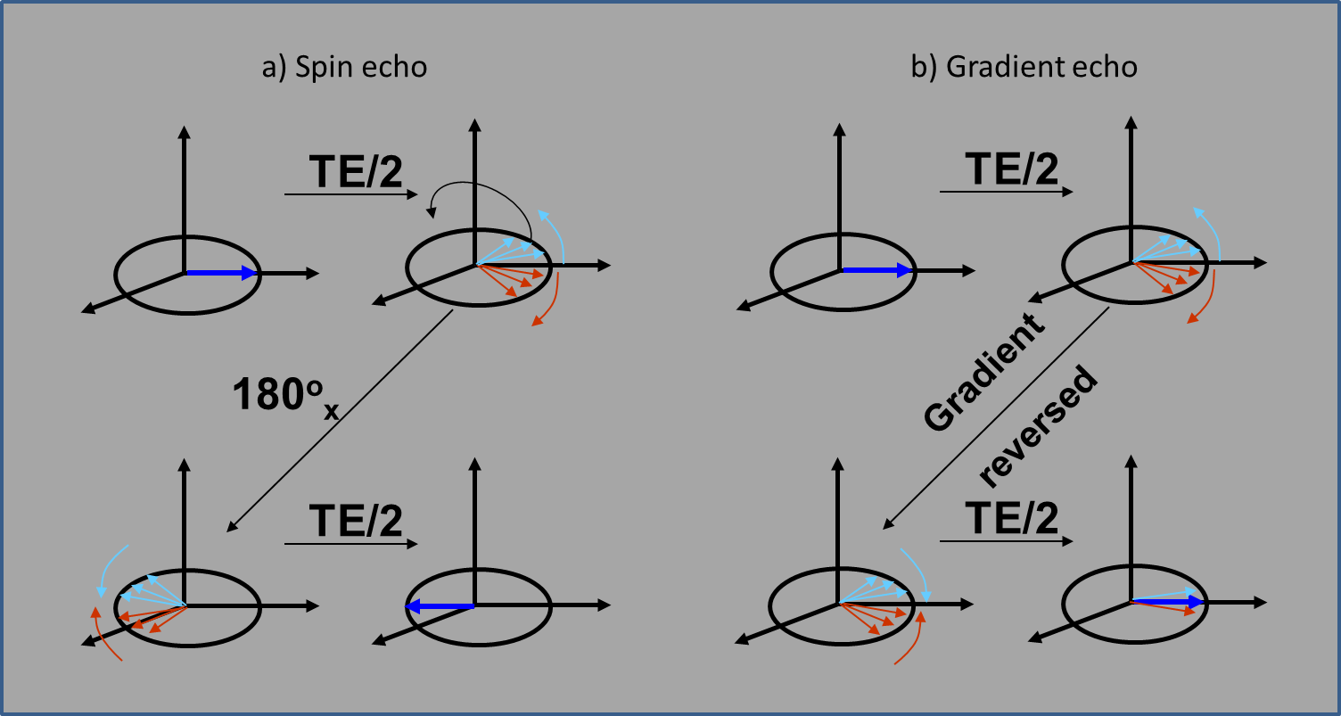
Spin Echo imaging is the basis for many structural MRI (sMRI) sequences, and uses an extra (180^o) pulse to refocus effects of dephasing. As shown in Figure 3a, an initial 90^o pulse (along x') produces transverse magnetisation along y', which dephases due to variations (inhomogeneities) in the local magnetic field. Applying a 180^o pulse (along x') flips spins to a different (mirrored) position in the transverse plane, after which they continue to precess in same direction and at same speed as before (as they are still experiencing the same local magnetic field). The transverse magnetisation therefore rephases along the -y’ axis, producing an echo signal that reaches a maximum at the echo time, TE, before decaying away again.

Gradient Echo imaging, which creates an echo without using a 180^o pulse, is used for both structural and functional MRI (fMRI). As shown in Figure 3b, an initial excitation pulse (show here as a 90^o pulse (along x'), although lower flip angles can also be used) produces transverse magnetisation along y', in the same way as for a spin echo. If a magnetic field gradient is now applied, the transverse magnetisation will dephase due to both time-invariant local field inhomogeneities (as in the spin echo case) and the applied gradient. If the gradient is then reversed, spins will precess in opposite direction and at (almost) the same speed as before, so that the transverse magnetisation rephases, again producing an echo signal that reaches a maximum at the echo time, TE, before decaying away again. Since for the effect of local inhomogeneities remains the same throughout the whole TE period, however (in contrast to the applied gradient, which is positive during one half of TE and negative during the other), the effect of local inhomogeneities is NOT refocused.

Putting it all together...

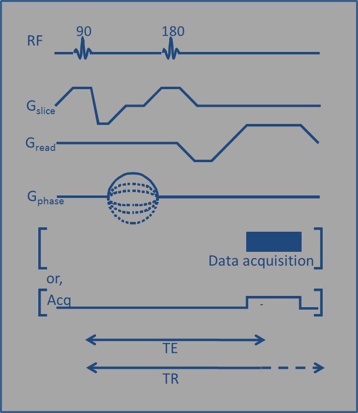
A Pulse Sequence Diagram (e.g. Figure 4, which shows a spin echo sequence) can be used to diagrammatically show all gradients & RF pulses that are applied in order to form an image. It shows the relative timing and amplitudes of each pulse, but may not be drawn exactly to scale. Shading is often used to indicate gradient areas which should be equal (or equal and opposite), with arrows indicating exact timing of events (in particular TE, the Echo Time and TR, the Repetition Time (i.e. the length of time between applying the first excitation pulse in a sequence, and repeating this (for signal averaging, or to collect the next phase encode step)).

Relaxation and Image Contrast

Relaxation

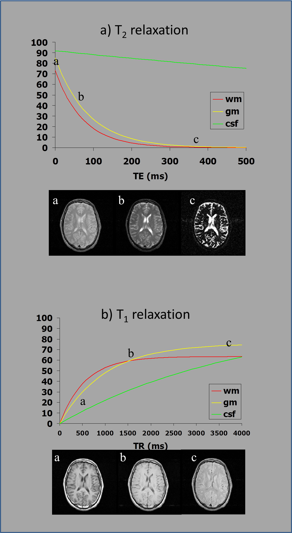
After we disturb the magnetisation in any way, it relaxes back to its original configuration. This effect is described by two main time constants, T₁ and T₂ . (We’ll also mention T₂^*). These relaxation times are fundamental MR parameters reflecting the ‘tissue environment’ (the binding and mobility of water within tissues). Along with PD (the proton density), T₁ and T₂ are responsible for (most) contrast in MR images; different combinations of TE and TR can be used to produce different degrees of contrast (intensity difference) between tissues, with changes of TR leading to changes in contrast between tissues with different T₁ relaxation times, and changes in TE changing contrast between tissues with different T₂s.

Mathematically, for a spin echo sequence:

$$I_{SE} = g PD \exp{\left(- \frac {TE} {T_2} \right)} \left[ 1 - \exp{\left(- \frac {TR} {T_1} \right)} \right]$$

(A similar equations holds for some gradient echo sequences, with T₂ being replaced by T₂^* to reflect the difference in signal loss due to dephasing in local field inhomogenities).

Relaxation Times

T₁ is known as the Longitudinal or Spin-lattice relaxation time, and describes the return of the net magnetisation towards its equilibrium position (parallel to B₀) after it has been disturbed (e.g. by a 90^o pulse flipping it into the transverse plane). T₁ is time taken for z- magnetisation to recover to 67% of its initial value following a 90^o pulse. It varies between tissues and T₁ contrast often gives good differentiation of anatomical structures. (Figure 5a).

T₂ (the Transverse or Spin-spin relaxation time) also varies between tissues, and is often (non-specifically) increased in pathological regions. After excitation, any differences in the local magnetic field the experience will lead to spins precessing at different frequencies; the overall net transverse magnetisation will therefore dephase, and the measured signal will decrease. (Figure 5b). T₂ is time taken for signal to decay, in a homogenous static magnetic field, to 37% of its initial value, while T₂^* is the equivalent time in an inhomogeneous field.

The Bloch Equations

The Bloch equations give complete classical description of the behaviour of magnetisation under influence of an applied field, and of relaxation. The applied field can include:

• any B_z present in rotating frame (i.e. off-resonance effects)
• field gradients (which may vary with time)
• the RF field B₁ (which may be applied x' or y' axis, or a combination, and may vary with time)

Precession of M around B is described by:

$$\frac{\partial M}{\partial t} = \gamma M \times B$$

... which expands to:

$$\frac{\partial M_x}{\partial t} = \gamma \left(M_y B_z - M_z B_y\right)$$

$$\frac{\partial M_y}{\partial t} = \gamma \left(M_z B_x - M_x B_y\right)$$

$$\frac{\partial M_z}{\partial t} = \gamma \left(M_x B_y - M_y B_x\right)$$

Relaxation is dealt with by additional (phenomenological) terms:

$$\frac{\partial M_x}{\partial t} = \gamma \left(M_y B_z - M_z B_y\right) - \frac {M_x} {T_2} $$

$$\frac{\partial M_y}{\partial t} = \gamma \left(M_z B_x - M_x B_y\right) - \frac {M_y} {T_2} $$

$$\frac{\partial M_z}{\partial t} = \gamma \left(M_x B_y - M_y B_x\right) + - \frac {M_0 - M_z} {T_1} $$

... and other terms can also be added (e.g. to allow for diffusion or other weightings).

Summary

• Quantum Mechanics says that some nuclei will have angular momentum, or “spin”; this includes protons (hydrogen nuclei).
• Spinning, charged, particles create a (tiny) magnetic field, so hydrogen nuclei - in water, and organic molecules - have a magnetic moment (much like a bar magnet).
• In a magnetic field, such NMR visible nuclei align themselves with direction of the magnetic field (B₀), some “up” and some “down”; the overall effect of all up and down spins can be though of in terms of a single net magnetisation, M.
• M behaves like a gyroscope and precesses around magnetic field (B₀) at the Larmor frequency, $$$\omega_0 = \gamma B_0$$$.
• If ‘flipped’ into transverse plane, M induces a detectable voltage in surrounding conductors.Gradients for allow us to spatially localise this signal, forming an image.
• Differences in relaxation times determine how much signal we measure, allowing us to manipulate image contrast.
• The Bloch equations allow the overall magnetisation at any time to be calculated, allowing for effects of RF pulses, relaxation, etc.

Conclusions

Acknowledgements

References

[1] E. M. Purcell, H. C. Torrey, and R. V. Pound, Resonance Absorption by Nuclear Magnetic Moments in a Solid. Phys. Rev. 69, 37 (1946)

[2] F. Bloch, W. W. Hansen, and M. Packard. The Nuclear Induction Experiment. Phys. Rev. 70, 474 (1946)

[3] T. Farrar and E. Becker, Pulse and Fourier Transform NMR. Introduction to Theory and Method, Elsevier, (1971)

[4] F. Bloch, Nuclear Induction, Phys. Rev. 70, 460 (1946)