Susceptibility Mapping in Brain Diseases: Iron, Myelin & More
Synopsis
Tissue magnetic susceptibility can be calculated from gradient-echo phase images using quantitative susceptibility mapping (QSM). Several clinical applications of QSM are emerging based on its sensitivity to tissue iron, myelin and deoxyhaemoglobin content. These include visualising iron in deep-brain structures in Parkinson’s disease and other dementias, evaluating microbleed burden and haemorrhages and distinguishing these from calcifications. QSM also allows quantification of venous oxygenation with functional QSM now able to detect brain activity. QSM reveals demyelination: changes in both myelin and iron content drive QSM differences in Multiple Sclerosis which may be associated with inflammation, perhaps due to iron in microglia/macrophages.
What is Susceptibility?
Susceptibility is an intrinsic bulk material or tissue property that determines how a material or tissue will interact with and behave in an applied magnetic field [1]. Tissues with positive susceptibility values are paramagnetic (i.e. their magnetisation increases with the applied magnetic field strength) and those with negative susceptibility values are diamagnetic. The reason we are interested in tissue magnetic susceptibility is that it is directly related to the tissue composition and microstructure. This means susceptibility maps have the potential to yield interesting information on pathophysiology-related changes in tissue composition and microstructure, particularly in the brain.How Can We Measure Tissue Magnetic Susceptibility?
Now that we have established that susceptibility depends on tissue composition, how might we actually measure this tissue magnetic susceptibility ($$$\chi$$$)? The key to this is that the phase of the complex MRI signal in simple T2*-weighted gradient-echo MRI sequences is directly determined by the underlying tissue magnetic susceptibility [2, 3]. It is useful to picture a small spherical point ‘source’ with a different susceptibility to its surroundings, in a magnetic field (B0 along the z direction). The source will produce small magnetic field perturbations that have a dipolar distribution (d(r)) (Figure 1). A more complicated susceptibility distribution $$$\chi$$$(r) will lead to a more complicated field distribution ΔBz(r) which can be understood as the sum or superposition of many dipole fields from many small point sources of susceptibility. This can be expressed mathematically as follows:
$$B_z(r) = B_0 . d(r)\otimes \chi(r)$$ (1)
which means that, if we knew the susceptibility distribution inside tissue ($$$\chi$$$(r)) it would be possible to calculate the field distribution ΔBz(r) by convolving $$$\chi$$$(r) with the unit dipole field kernel d(r).
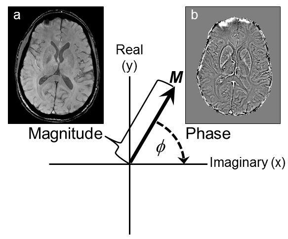
We are able to measure the field perturbations induced by tissue magnetic susceptibility distributions because they are linearly related to the phase of the complex MRI signal in T2*-weighted gradient-echo MRI sequences. The phase φ(r) is related to ΔBz(r) according to
$$ \phi(r,TE) = \gamma\triangle B_z(r).TE + \phi_0(r)$$ (2)
where γ is the gyromagnetic ratio, TE is the echo time and φ0(r) is the phase at TE=0 (Figure 2). This means that the rich contrast available in these phase images [4], which were often discarded in the past, can be used to calculate (based on equations 1 and 2) maps of the underlying tissue magnetic susceptibility distribution. The problem with using phase images as they are is that the phase contrast is non-local, extending beyond the structures of interest, and also depends on the orientation of these structures with respect to the main magnetic field B0. Susceptibility Mapping overcomes these disadvantages [5].
Stages in QSM
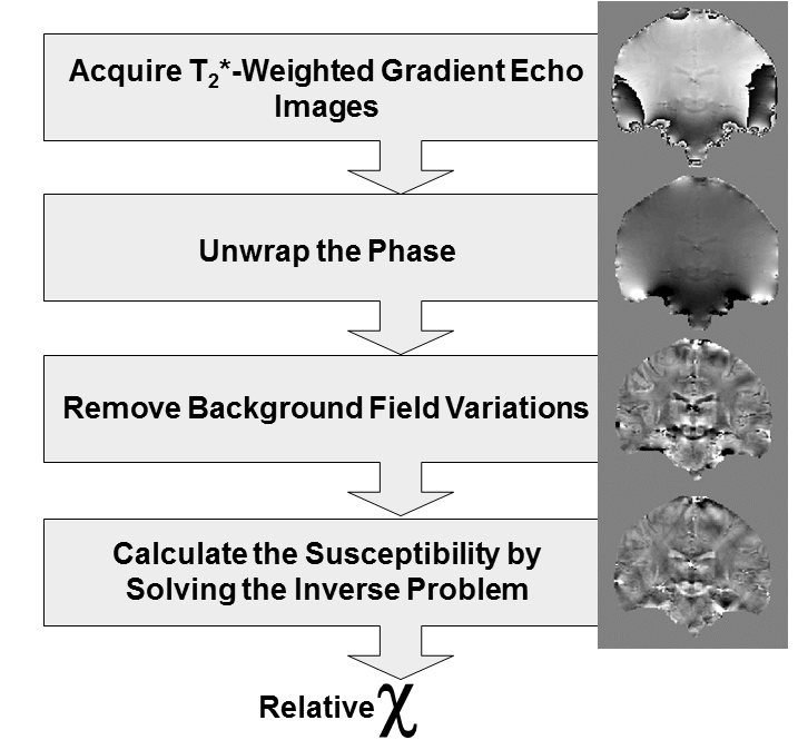
This process of susceptibility mapping (often called Quantitative Susceptibility Mapping (QSM), Figure 3) has developed rapidly over the last few years and has been described in several recent review papers [6-9]. The conceptual steps in QSM are shown in Figure 3 and can be summarized as follows. the first step is acquisition of T2*-Weighted gradient echo images, taking care to save the complex (magnitude and phase) images. When using multiple channel radio frequency coils, it is crucial to ensure that the phase images from each of the coil channels is combined correctly to reconstruct an accurate phase image [10-13] otherwise intractable artifacts known as open-ended fringe lines or phase singularities can occur. It is also important to obtain the most accurate estimate of ΔBz(r) by fitting over phase images φ(r,TE) measured at multiple echo times [14, 15]. The next step is to unwrap the phase images for which there are a large variety of unwrapping algorithms available, e.g. [16-18], each with their own advantages and drawbacks. This is followed by removal of large-scale background phase variations caused primarily by the relatively large susceptibility difference between tissue and air in cavities and outside the body. These background phase variations are often much larger than the susceptibility-induced phase differences of interest between different tissues and there are now a wide variety of techniques for removing them, e.g. [19-21]. Masking out noisy phase in areas where there is no MRI signal (e.g. outside the body) is often a prerequisite for applying (unwrapping and) background field removal. It is important to note that, as a result of removing background phase variations, the contrast observed in susceptibility maps is relative rather than absolute.
The final step in calculating susceptibility images from these processed phase images is to solve the inverse problem i.e. calculate the susceptibility distribution χ(r) from the measured phase images φ(r). A large variety of methods have been developed to overcome this ill-posed, ill-conditioned inverse problem or regularize it. Although we have described several separate conceptual steps in QSM. Practically or computationally, these may often be combined into fewer steps [22, 23] or even a single step [24].
The key message is that there are now a large variety of QSM algorithms available, each one with its own relative merits and disadvantages. The tissue magnetic susceptibility maps produced using these methods have important advantages over the phase images from which they were calculated; they overcome the non-local and orientation-dependent nature of the contrast in phase images [5], allowing improvements in the visualisation of tissue structure and composition. These advantages also stand against the earlier and more widespread precursor to QSM known as susceptibility weighted imaging (SWI) in which phase images are unwrapped, filtered and multiplied with the corresponding magnitude images to emphasise susceptibility-induced phase changes [25]. A common practical pitfall is the acquisition of images with insufficient resolution and/or coverage [8, 26, 27] for QSM. It is important to ensure that the field perturbations ΔBz(r) induced by susceptibility sources χ(r) are sufficiently sampled so that they can be accurately inverted.
Why? QSM Contrast Sources and Applications in the Brain
The dominant sources of contrast in susceptibility maps [28] are widely accepted to be tissue iron and myelin content as well as calcifications and deoxyhaemoglobin in blood vessels. Tissue susceptibility is also affected by tissue microstructure and compartmentalisation and the susceptibility in white matter has been found to be anisotropic [29-31].
Tissue Iron – Deep-Brain Structures and Dementia
Tissues rich in ferritin (stored iron) are relatively paramagnetic and show strong contrast in susceptibility maps. Several investigators have found strong correlations between the measured tissue magnetic susceptibility in brain regions such as the red nucleus, substantia nigra and putamen and their iron content, often estimated from post-mortem studies [19, 32-34]. Tissue MRI susceptibility values have also been found to correlate with iron content measured in the same tissue using independent methods such as X-ray fluorescence imaging and inductively coupled plasma mass spectrometry [35, 36]. The dependence of susceptibility image contrast on tissue iron content has been exploited for several clinical applications in the brain, for example to improve targeting of structures for deep-brain stimulation [37-39] and as a marker of increased iron content in the substantia nigra in patients with Parkinson’s disease (PD) [40-49]. SM has also been applied in Alzheimer’s Disease (AD) in which the characteristic amyloid beta protein plaques have been found to co-localise with iron [50, 51]. SM has shown promise for identifying plaques in fixed brain specimens from patients with AD [52]. Initial SM studies in patients with early-stage AD [50, 53, 54] found susceptibility differences in both deep grey matter and cortical regions. SM studies in animal models of AD have also shown structural differences including increased microbleed load [55] and susceptibility increases associated with demyelination in the corpus callosum and other regions [56]. Therefore, SM shows exciting potential to provide imaging biomarkers to facilitate early diagnosis of PD and AD. Recent studies have also used susceptibility mapping to measure subcortical iron accumulation in Huntington’s disease [57, 58], subcortical copper and/or iron accumulation in the brain in Wilson disease [59] and iron in the motor cortex in Amyotrophic Lateral Sclerosis [60].
Deoxyhaemoglobin and Blood Iron – Brain Oxygenation and Microvascular disease
It is well-established that deoxyhaemoglobin is paramagnetic with respect to most tissues and this is the basis of functional MRI and susceptibility-weighted imaging (SWI) [7, 25]. Because deoxyhaemoglobin is paramagnetic, susceptibility maps highlight the venous vasculature [61] and because the venous susceptibility depends linearly on the deoxyhaemoglobin concentration, susceptibility mapping allows quantification of venous oxygenation [62-66]. The high paramagnetic susceptibility of deoxyhaemoglobin and other blood products (e.g. haemosiderin) has also enabled susceptibility maps to reveal and assess haemorrhages and microbleeds [55, 67-69], for example in traumatic brain injury [70, 71]. A further advantage of susceptibility mapping over phase imaging or SWI is that these strongly paramagnetic haemorrhages and microbleeds can be easily distinguished from calcifications in susceptibility maps [72-75] as calcium compounds are strongly diamagnetic. A further emerging application is the utilisation of endogenous oxygenation-dependent susceptibility contrast for functional imaging [76-78] in so-called fQSM.
Myelin – Demyelination
In addition to revealing paramagnetic contributions, susceptibility maps also show prominent diamagnetic sources including myelin which is thought to have a slightly more diamagnetic susceptibility than other tissues due to its high lipid content [4, 79]. Demyelination, induced by a cuprizone diet [79] or in shiverer mice [80], has been shown to almost completely remove the susceptibility-induced contrast between grey and white matter. QSM has also been used to reveal demyelination in a model of tau pathology [56]. Changes in the susceptibility contrast in and around Multiple Sclerosis (MS) lesions has been attributed to changes in both myelination and iron content [10, 81-90] as well as microstructural alterations and this is an active, and occasionally controversial, area of research [91-95].
Inflammation
It is likely that the iron deposition at the rim of white matter lesions in MS is in M1 microglia / macrophages which cause residual inflammation that remains even after the blood-brain barrier re-seals. Systemic lupus erythematosus (SLE) is a disease which involves inflammation and does not usually have observable correlates in MR images. QSM showed increased susceptibility in the putamen and globus pallidus of SLE patients relative to healthy controls [96], suggesting that iron accumulates as a result of the pathophysiology of the disease, probably including inflammation.
Microstructure and Susceptibility Anisotropy
In addition to its composition, tissue’s structure at several different scales, orientational ordering and compartmentalisation [97] affect the susceptibility contrast. Even if a tissue structure’s overall macroscopic shape and geometry remain constant, if its microstructural orientation with respect to B0 is altered, this changes the phase contrast and correspondingly the calculated magnetic susceptibility [29]. This phenomenon has been explained by susceptibility anisotropy [98, 99], such that susceptibility can be understood as a tensor. Susceptibility anisotropy has been measured in white matter (whose fibres are found to be more diamagnetic when they run perpendicular to B0) and seems to arise from the highly ordered macro-molecular structure of the lipid bilayers in the myelin sheath [31]. This effect has been exploited in Susceptibility Tensor Imaging [30, 98, 100-102] to reveal white matter structure via a mechanism complementary to that utilised in Diffusion Tensor Imaging. However, this is unlikely to translate into the clinic as it requires imaging of the head at multiple orientations relative to B0 which is uncomfortable and time-consuming.
Thanks to its ability to reveal multiple pathophysiologically important tissue components, QSM is likely to be increasingly used to assess tissue composition and microstructure in a variety of brain diseases [103].
Acknowledgements
No acknowledgement found.References
[1] J.F. Schenck, The role of magnetic susceptibility in magnetic resonance imaging: MRI magnetic compatibility of the first and second kinds. Medical Physics, 1996. 23(6): 815-850. [2] J.P. Marques and R. Bowtell, Application of a Fourier-based method for rapid calculation of field inhomogeneity due to spatial variation of magnetic susceptibility. Concepts in Magnetic Resonance Part B: Magnetic Resonance Engineering, 2005. 25B(1): 65-78. [3] R. Salomir, et al., A fast calculation method for magnetic field inhomogeneity due to an arbitrary distribution of bulk susceptibility. Concepts in Magnetic Resonance Part B-Magnetic Resonance Engineering, 2003. 19B(1): 26-34. [4] J.H. Duyn, et al., High-field MRI of brain cortical substructure based on signal phase. Proc Natl Acad Sci U S A, 2007. 104(28): 11796-801. [5] K. Shmueli, et al. The Dependence of Tissue Phase Contrast on Orientation Can Be Overcome by Quantitative Susceptibility Mapping. in Proc ISMRM, 2009. Honolulu, Hawai'i, USA, 17, p. 466. [6] Y. Wang and T. Liu, Quantitative susceptibility mapping (QSM): Decoding MRI data for a tissue magnetic biomarker. Magn Reson Med, 2014.In Press. [7] C. Liu, et al., Susceptibility-weighted imaging and quantitative susceptibility mapping in the brain. J Magn Reson Imaging, 2015. 42(1): 23-41. [8] E.M. Haacke, et al., Quantitative susceptibility mapping: current status and future directions. Magn Reson Imaging, 2015. 33(1): 1-25. [9] A. Deistung, et al., Overview of quantitative susceptibility mapping. NMR in Biomedicine, 2016.In Press: n/a-n/a. [10] K.E. Hammond, et al., Development of a robust method for generating 7.0 T multichannel phase images of the brain with application to normal volunteers and patients with neurological diseases. Neuroimage, 2008. 39(4): 1682-92. [11] S. Robinson, et al., Combining Phase Images From Multi-Channel RF Coils Using 3D Phase Offset Maps Derived From a Dual-Echo Scan. Magnetic Resonance in Medicine, 2011. 65(6): 1638-1648. [12] D.L. Parker, et al., Phase Reconstruction from Multiple Coil Data Using a Virtual Reference Coil. Magnetic Resonance in Medicine, 2014. 72(2): 563-569. [13] S.D. Robinson, et al., Combining phase images from array coils using a short echo time reference scan (COMPOSER). Magn Reson Med, 2017. 77(1): 318-327. [14] E. Biondetti, et al. Application of Laplacian-based Methods to Multi-echo Phase Data for Accurate Susceptibility Mapping. in Proc ISMRM, 2016. Singapore, 24, p. 1547. [15] T. Liu, et al., Nonlinear formulation of the magnetic field to source relationship for robust quantitative susceptibility mapping. Magn Reson Med, 2013. 69: 467-476. [16] M. Jenkinson, Fast, automated, N-dimensional phase-unwrapping algorithm. Magnetic Resonance in Medicine, 2003. 49(1): 193. [17] S. Witoszynskyj, et al., Phase unwrapping of MR images using Phi UN - A fast and robust region growing algorithm. Medical Image Analysis, 2009. 13(2): 257-268. [18] M.A. Schofield and Y.M. Zhu, Fast phase unwrapping algorithm for interferometric applications. Optics Letters, 2003. 28(14): 1194-1196. [19] F. Schweser, et al., Quantitative imaging of intrinsic magnetic tissue properties using MRI signal phase: an approach to in vivo brain iron metabolism? Neuroimage, 2011. 54(4): 2789-807. [20] T. Liu, et al., A novel background field removal method for MRI using projection onto dipole fields (PDF). NMR in Biomedicine, 2011. 24(9): 1129-1136. [21] F. Schweser, et al., An illustrated comparison of processing methods for phase MRI and QSM: removal of background field contributions from sources outside the region of interest. NMR in Biomedicine, 2016.In Press. [22] F. Schweser, et al., Toward online reconstruction of quantitative susceptibility maps: superfast dipole inversion. Magn Reson Med, 2013. 69(6): 1582-94. [23] W. Li, et al., Integrated Laplacian-based phase unwrapping and background phase removal for quantitative susceptibility mapping. NMR Biomed, 2014. 27(2): 219-27. [24] I. Chatnuntawech, et al., Single-step quantitative susceptibility mapping with variational penalties. NMR in Biomedicine, 2016.In Press: n/a-n/a. [25] E.M. Haacke, et al., Susceptibility weighted imaging (SWI). Magn Reson Med, 2004. 52(3): 612-8. [26] A. Karsa, et al. The Effect of Large Slice Thickness and Spacing and Low Coverage on the Accuracy of Susceptibility Mapping. in Proc ISMRM, 2016. Singapore, 24, p. 1555. [27] A.M. Elkady, et al., Importance of extended spatial coverage for quantitative susceptibility mapping of iron-rich deep gray matter. Magnetic Resonance Imaging. 34(4): 574-578. [28] J.H. Duyn and J. Schenck, Contributions to magnetic susceptibility of brain tissue. NMR in Biomedicine, 2016.In Press: n/a-n/a. [29] J. Lee, et al., Sensitivity of MRI resonance frequency to the orientation of brain tissue microstructure. Proc Natl Acad Sci U S A, 2010. 107(11): 5130-5. [30] W. Li, et al., Susceptibility tensor imaging (STI) of the brain. NMR Biomed, 2016.In Press. [31] W. Li, et al., Magnetic susceptibility anisotropy of human brain in vivo and its molecular underpinnings. NeuroImage, 2012. 59(3): 2088-2097. [32] K. Shmueli, et al., Magnetic susceptibility mapping of brain tissue in vivo using MRI phase data. Magn Reson Med, 2009. 62(6): 1510-22. [33] F. Schweser, et al., SEMI-TWInS: Simultaneous Extraction of Myelin and Iron using a T2*-Weighted Imaging Sequence. Proceedings 19th Scientific Meeting, International Society for Magnetic Resonance in Medicine, 2011.In Press: 120. [34] S. Wharton and R. Bowtell, Whole-brain susceptibility mapping at high field: a comparison of multiple- and single-orientation methods. Neuroimage, 2010. 53(2): 515-25. [35] C. Langkammer, et al., Quantitative susceptibility mapping (QSM) as a means to measure brain iron? A post mortem validation study. Neuroimage, 2012. 62(3): 1593-1599. [36] W.L. Zheng, et al., Measuring iron in the brain using quantitative susceptibility mapping and X-ray fluorescence imaging. Neuroimage, 2013. 78: 68-74. [37] R.L. O'Gorman, et al., Optimal MRI methods for direct stereotactic targeting of the subthalamic nucleus and globus pallidus. Eur Radiol, 2011. 21(1): 130-6. [38] T. Liu, et al., Improved Subthalamic Nucleus Depiction with Quantitative Susceptibility Mapping. Radiology, 2013. 269(1): 216-223. [39] A.S. Chandran, et al., Magnetic resonance imaging of the subthalamic nucleus for deep brain stimulation. Journal of Neurosurgery, 2016. 124(1): 96-105. [40] A.K. Lotfipour, et al., High resolution magnetic susceptibility mapping of the substantia nigra in Parkinson's disease. J Magn Reson Imaging, 2012. 35(1): 48-55. [41] Y. Murakami, et al., Usefulness of Quantitative Susceptibility Mapping for the Diagnosis of Parkinson Disease. AJNR Am J Neuroradiol, 2015.In Press. [42] J. Acosta-Cabronero, et al., The whole-brain pattern of magnetic susceptibility perturbations in Parkinson’s disease. Brain, 2016.In Press. [43] C. Langkammer, et al., Quantitative Susceptibility Mapping in Parkinson's Disease. Plos One, 2016. 11(9). [44] M. Azuma, et al., Lateral Asymmetry and Spatial Difference of Iron Deposition in the Substantia Nigra of Patients with Parkinson Disease Measured with Quantitative Susceptibility Mapping. American Journal of Neuroradiology, 2016. 37(5): 782-788. [45] N.Y. He, et al., Region-specific disturbed iron distribution in early idiopathic Parkinson's disease measured by quantitative susceptibility mapping. Human Brain Mapping, 2015. 36(11): 4407-4420. [46] G.W. Du, et al., Quantitative susceptibility mapping of the midbrain in Parkinson's disease. Movement Disorders, 2016. 31(3): 317-324. [47] J.H.O. Barbosa, et al., Quantifying brain iron deposition in patients with Parkinson's disease using quantitative susceptibility mapping, R2 and R2. Magnetic Resonance Imaging, 2015. 33(5): 559-565. [48] S. Ide, et al., Internal structures of the globus pallidus in patients with Parkinson’s disease: evaluation with quantitative susceptibility mapping (QSM). European Radiology, 2014. 25(3): 710-718. [49] X. Guan, et al., Regionally progressive accumulation of iron in Parkinson's disease as measured by quantitative susceptibility mapping. NMR in Biomedicine, 2016.In Press. [50] J.M. van Bergen, et al., Colocalization of cerebral iron with Amyloid beta in Mild Cognitive Impairment. Sci Rep, 2016. 6: 35514. [51] M.A. Smith, et al., Increased iron and free radical generation in preclinical Alzheimer disease and mild cognitive impairment. J Alzheimers Dis, 2010. 19(1): 363-72. [52] M. Zeineh, et al. Susceptibility Mapping of Alzheimer Plaques at 7T. in Proc ISMRM, 2011. Montréal, Québec, Canada, 19, p. 586. [53] J. Acosta-Cabronero, et al., In Vivo Quantitative Susceptibility Mapping (QSM) in Alzheimer's Disease. Plos One, 2013. 8(11). [54] Y. Moon, et al., Patterns of Brain Iron Accumulation in Vascular Dementia and Alzheimer's Dementia Using Quantitative Susceptibility Mapping Imaging. J Alzheimers Dis, 2016. 51(3): 737-45. [55] J. Klohs, et al., Detection of cerebral microbleeds with quantitative susceptibility mapping in the ArcAbeta mouse model of cerebral amyloidosis. Journal of Cerebral Blood Flow and Metabolism, 2011. 31(12): 2282-2292. [56] J. O'Callaghan, et al. Does Tau Pathology Play a Role in Abnormal Iron Deposition in Alzheimer’s Disease? a Quantitative Susceptibility Mapping Study in the RTg4510 Mouse Model of Tauopathy. in Proc ISMRM, 2016. Singapore, 24, p. 3380. [57] J.M.G. Van Bergen, et al., Quantitative susceptibility mapping suggests altered brain iron in premanifest Huntington disease. American Journal of Neuroradiology, 2016. 37(5): 789-796. [58] J.F. Domínguez D, et al., Iron accumulation in the basal ganglia in Huntington's disease: Cross-sectional data from the IMAGE-HD study. Journal of Neurology, Neurosurgery and Psychiatry, 2016. 87(5): 545-549. [59] D. Fritzsch, et al., Seven-Tesla Magnetic Resonance Imaging in Wilson Disease Using Quantitative Susceptibility Mapping for Measurement of Copper Accumulation. Investigative Radiology, 2014. 49(5): 299-306. [60] A.D. Schweitzer, et al., Quantitative susceptibility mapping of the motor cortex in amyotrophic lateral sclerosis and primary lateral sclerosis. American Journal of Roentgenology, 2015. 204(5): 1086-1092. [61] S.F. Liu, et al., Improved MR Venography Using Quantitative Susceptibility-Weighted Imaging. Journal of Magnetic Resonance Imaging, 2014. 40(3): 698-708. [62] B. Xu, et al., Flow Compensated Quantitative Susceptibility Mapping for Venous Oxygenation Imaging. Magnetic Resonance in Medicine, 2014. 72(2): 438-445. [63] A.P. Fan, et al., Quantitative oxygenation venography from MRI phase. Magn Reson Med, 2014. 72(1): 149-59. [64] M.C. Hsieh, et al., Investigating hyperoxic effects in the rat brain using quantitative susceptibility mapping based on MRI phase. Magn Reson Med, 2016.In Press. [65] M.C. Hsieh, et al., Quantitative Susceptibility Mapping-Based Microscopy of Magnetic Resonance Venography (QSM-mMRV) for In Vivo Morphologically and Functionally Assessing Cerebromicrovasculature in Rat Stroke Model. PLoS One, 2016. 11(3): e0149602. [66] F.W. Wehrli, et al., Susceptibility-based time-resolved whole-organ and regional tissue oximetry. NMR in Biomedicine, 2016.In Press. [67] J. Klohs, et al., Longitudinal Assessment of Amyloid Pathology in Transgenic ArcA beta Mice Using Multi-Parametric Magnetic Resonance Imaging. Plos One, 2013. 8(6). [68] T. Liu, et al., Cerebral Microbleeds: Burden Assessment by Using Quantitative Susceptibility Mapping. Radiology, 2012. 262(1): 269-278. [69] H. Tan, et al., Evaluation of iron content in human cerebral cavernous malformation using quantitative susceptibility mapping. Investigative Radiology, 2014. 49(7): 498-504. [70] W. Liu, et al., Imaging cerebral microhemorrhages in military service members with chronic traumatic brain injury. Radiology, 2016. 278(2): 536-545. [71] K. Chary, et al. Quantitative susceptibility mapping of the rat brain after traumatic brain injury. in Proceedings of the 24th Annual Meeting of the International Society for Magnetic Resonance in Medicine, 2016. Singapore, 24, p. 34. [72] F. Schweser, et al., Differentiation between diamagnetic and paramagnetic cerebral lesions based on magnetic susceptibility mapping. Med Phys, 2010. 37(10): 5165-78. [73] F. Schweser, et al., Quantitative magnetic susceptibility mapping (QSM) in breast disease reveals additional information for MR-based characterization of carcinoma and calcification. Proceedings 19th Scientific Meeting, International Society for Magnetic Resonance in Medicine, 2011.In Press: 1014. [74] A. Deistung, et al., Quantitative Susceptibility Mapping Differentiates between Blood Depositions and Calcifications in Patients with Glioblastoma. Plos One, 2013. 8(3). [75] W. Chen, et al., Intracranial calcifications and hemorrhages: Characterization with quantitative susceptibility mapping. Radiology, 2014. 270(2): 496-505. [76] D.Z. Balla, et al., Functional quantitative susceptibility mapping (fQSM). Neuroimage, 2014. 100: 112-124. [77] M. Bianciardi, et al., Investigation of BOLD fMRI resonance frequency shifts and quantitative susceptibility changes at 7 T. Human Brain Mapping, 2014. 35(5): 2191-2205. [78] J.R. Reichenbach, The future of susceptibility contrast for assessment of anatomy and function. Neuroimage, 2012. 62(2): 1311-5. [79] J. Lee, et al., The contribution of myelin to magnetic susceptibility-weighted contrasts in high-field MRI of the brain. Neuroimage, 2012. 59(4): 3967-75. [80] C.L. Liu, et al., High-field (9.4 T) MRI of brain dysmyelination by quantitative mapping of magnetic susceptibility. Neuroimage, 2011. 56(3): 930-938. [81] D.A. Yablonskiy, et al., Biophysical mechanisms of MRI signal frequency contrast in multiple sclerosis. Proceedings of the National Academy of Sciences of the United States of America, 2012. 109(35): 14212-14217. [82] B. Yao, et al., Chronic Multiple Sclerosis Lesions: Characterization with High-Field-Strength MR Imaging. Radiology, 2012. 262(1): 206-215. [83] C. Langkammer, et al., Quantitative susceptibility mapping in multiple sclerosis. Radiology, 2013. 267(2): 551-9. [84] W. Chen, et al., Quantitative susceptibility mapping of multiple sclerosis lesions at various ages. Radiology, 2014. 271(1): 183-92. [85] C. Wisnieff, et al., Quantitative susceptibility mapping (QSM) of white matter multiple sclerosis lesions: Interpreting positive susceptibility and the presence of iron. Magn Reson Med, 2015. 74(2): 564-70. [86] S. Eskreis-Winkler, et al., Multiple sclerosis lesion geometry in quantitative susceptibility mapping (QSM) and phase imaging. J Magn Reson Imaging, 2015. 42(1): 224-9. [87] Y. Zhang, et al., Longitudinal change in magnetic susceptibility of new enhanced multiple sclerosis (MS) lesions measured on serial quantitative susceptibility mapping (QSM). J Magn Reson Imaging, 2016. 44(2): 426-32. [88] C. Stuber, et al., Iron in Multiple Sclerosis and Its Noninvasive Imaging with Quantitative Susceptibility Mapping. Int J Mol Sci, 2016. 17(1). [89] X. Li, et al., Magnetic susceptibility contrast variations in multiple sclerosis lesions. J Magn Reson Imaging, 2016. 43(2): 463-73. [90] M.J. Cronin, et al., A comparison of phase imaging and quantitative susceptibility mapping in the imaging of multiple sclerosis lesions at ultrahigh field. MAGMA, 2016. 29(3): 543-57. [91] D.A. Yablonskiy, et al., Lorentz Sphere Versus Generalized Lorentzian Approach: What Would Lorentz Say About It? Magnetic Resonance in Medicine, 2014. 72(1): 4-7. [92] D.A. Yablonskiy and A.L. Sukstanskii, Biophysical Mechanisms of Myelin-Induced Water Frequency Shifts. Magnetic Resonance in Medicine, 2014. 71(6): 1956-1958. [93] A.L. Sukstanskii and D.A. Yablonskiy, On the Role of Neuronal Magnetic Susceptibility and Structure Symmetry on Gradient Echo MR Signal Formation. Magnetic Resonance in Medicine, 2014. 71(1): 345-353. [94] J.H. Duyn and T.M. Barbara, Sphere of Lorentz and Demagnetization Factors in White Matter. Magnetic Resonance in Medicine, 2014. 72(1): 1-3. [95] J.H. Duyn, Frequency Shifts in the Myelin Water Compartment. Magnetic Resonance in Medicine, 2014. 71(6): 1953-1955. [96] A. Ogasawara, et al., Quantitative susceptibility mapping in patients with systemic lupus erythematosus: detection of abnormalities in normal-appearing basal ganglia. European Radiology, 2016. 26(4): 1056-1063. [97] W.C. Chen, et al., Detecting microstructural properties of white matter based on compartmentalization of magnetic susceptibility. Neuroimage, 2013. 70: 1-9. [98] C. Liu, Susceptibility tensor imaging. Magn Reson Med, 2010. 63(6): 1471-7. [99] D.A. Yablonskiy and A.L. Sukstanskii, Effects of biological tissue structural anisotropy and anisotropy of magnetic susceptibility on the gradient echo MRI signal phase: theoretical background. NMR Biomed, 2016.In Press. [100] C. Liu, et al., 3D fiber tractography with susceptibility tensor imaging. NeuroImage, 2012. 59(2): 1290-1298. [101] S. Wharton and R. Bowtell, Fiber orientation-dependent white matter contrast in gradient echo MRI. Proceedings of the National Academy of Sciences, 2012. 109(45): 18559-18564. [102] R. Dibb and C. Liu, Joint eigenvector estimation from mutually anisotropic tensors improves susceptibility tensor imaging of the brain, kidney, and heart. Magn Reson Med, 2016.In Press. [103] S. Eskreis-Winkler, et al., The clinical utility of QSM: disease diagnosis, medical management, and surgical planning. NMR in Biomedicine, 2016.In Press: n/a-n/a.Figures