5659
Fully Automated Left Ventricle Scar Quantification with Deep Learning1Technical University of Munich, Munich, Germany, 2Toronto General Hospital, University Health Network, Toronto, Canada, 3Department of Medicine, Beth Israel Deaconess Medical Center and Harvard Medical School, Boston, MA, United States
Synopsis
We present a fully automated approach for quantification of left ventricle scar in Late Gadolinium Enhancement (LGE) cardiac MR (CMR), using a residual neural network. LGE images were acquired in 1075 patients with known hypertrophic cardiomyopathy in a multi-center clinical trial. Scar segmentation was performed in all patients by a CMR-trained cardiologist. For training, we use a two-phase procedure, using cropped and full-sized images consecutively. We train different models using sigmoid cross-entropy loss and Dice loss and measure average LV segmentation Dice scores of 0.77 ± 0.10 and 0.70 ± 0.12 and estimated scar percentage mismatches of 3.59% and 3.00%, respectively.
Introduction
Late Gadolinium Enhancement (LGE) cardiac MR (CMR) is the standard technique for quantification of myocardial scar in the left ventricle (LV). Scar volume has important prognostic value and is often measured by manual contouring of scar boundaries. However, manual segmentation is time consuming and experience dependent. There have been numerous techniques developed over years to accurately calculate scar volume, however, these methods are often non-robust and require user interaction.1-4 In this paper, we sought to develop a fully automated approach for scar segmentation in the left ventricle based on deep learning.Methods
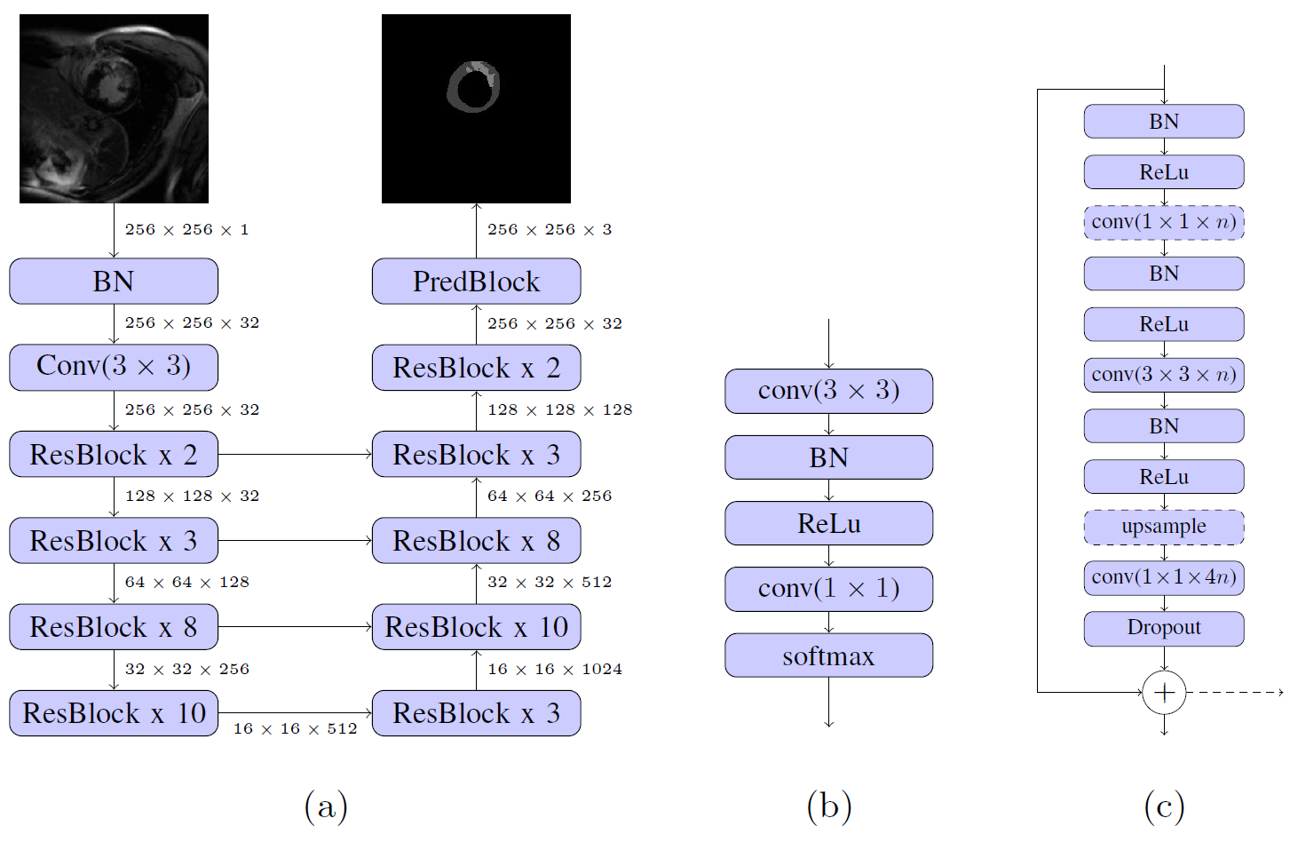
We propose to use a residual neural network architecture to automatically segment LV scar. A database consisting of 2D LGE images from 1075 patients with known hypertrophic cardiomyopathy acquired as part of a multi-center clinical trial was used to evaluate the performance of the approach.5 An experienced cardiologist with 5 years of experience in CMR manually segmented all images, which were used as “ground truth”.
A common problem in the segmentation of small objects, such as scar, is the high imbalance between background and foreground pixels, which is often tackled by elaborate loss-weighting schemes.6 We circumvent this challenge by applying a residual neural network architecture,7 which has shown competitive performance without weighted loss, when adapted for semantic segmentation.8 We set up our architecture (Figure 1) largely following these adaptions. Upsampling is realized by backwards-strided convolutions initialized for bilinear interpolation9 and dropout of 0.5 is applied in bottleneck layers during training.
We define the softmax cross-entropy loss
$$L_{x} = -\sum_{i} log(s_{i}^{c_{y}})\,,$$
using softmax probabilities $$$s_{i}^{c} \in [0,1]$$$ for classes $$$c \in \{0, 1, 2\}$$$ (background, healthy LV, scar), with $$$s_{i}^{c_{y}}$$$ being the softmax probability for the correct class at pixel $$$i$$$.
We define a second loss function, based on the Dice coefficient for the predicted segmentations:
$$L_{d} = \frac{1}{n}\sum_{c}(1 - \frac{2\sum_{i} s_{i}^{c} y_{i}^{c}}{\sum_{i} s_{i}^{c} + \sum_{i} y_{i}^{c}})\,.$$
Here, we calculate the average Dice loss for all $$$n$$$ classes, using softmax probabilities $$$s_{i}^{c}$$$ and ground truth label $$$y_i^{c}\in\{0,1\}$$$ for class $$$c$$$ at pixel $$$i$$$. Optimization is performed using the Adam method with learning rate of 0.001 and exponential decay rates $$$\beta_1$$$=1, $$$\beta_2$$$ = 0.999.10
The LGE images first undergo several preprocessing steps. Volumes are resampled to a pixel spacing of 1.2 mm and padded or cropped to a size of 256 x 256 pixels in the xy-plane. We augment training data by performing random translation, mirroring and elastic deformation on volumes during training.6 2D slices are used as input, after being normalized to zero mean and unit variance. We split the data into training and test sets, each containing 80% and 20% of the total data, respectively.
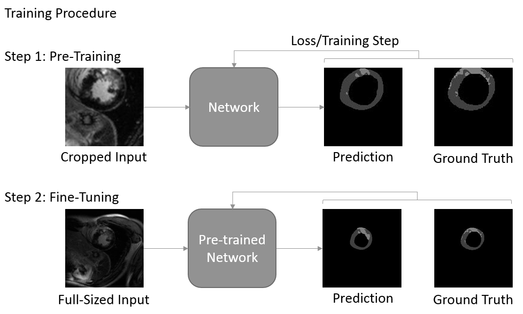
We follow a two-phase procedure for the training of the models (see Figure 1). First, the network is pre-trained with cropped, 128 x 128 sized patches that are extracted along the short axis of the heart. We train the network for up to 80000 iterations with batch size of 20. The best performing model is then fine-tuned for up to 20000 iterations with batch size 10 on full-sized images. By pre-training with cropped images, we reduce training time, while implicitly reducing the imbalance between background and foreground pixels. At test time, we apply a rectangular ROI filter on each volume to remove potential outliers.
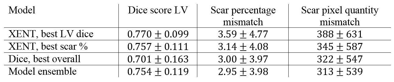
We perform quantitative evaluation on models generated with the different loss functions. In addition to the volume-wise LV Dice coefficient, we measure the accuracy of the predicted volume-wise scar percentage and pixel quantity. We evaluate two models trained with cross-entropy loss with best performance in LV segmentation and scar percentage prediction, respectively. Furthermore, we evaluate the model with best overall performance trained with Dice loss as well as an ensemble of all three models.
Results
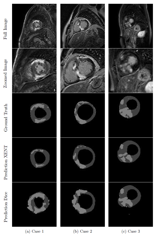
Figure 3 shows example scar segmentations achieved using the two approaches. LV dice scores were higher for models trained with cross-entropy loss, whereas the model trained with Dice loss achieves better scores for scar percentage estimation (see Table 1). Using an ensemble of the three individual models led to the best scar percentage estimation, while still achieving a high LV Dice score.Conclusion and Discussion
We present a new and robust method for fully automated scar quantification in LGE. Training and evaluation on a large-scale clinical data set shows good segmentation performance. In future work, further improvements could be made by incorporating the three-dimensionality of the data into the network architecture.11-14 While we did not apply any thresholding method for scar quantification in our work, the output of the network could be used to facilitate common scar thresholding methods.Acknowledgements
This work was supported by a fellowship within the FITweltweit programme of the German Academic Exchange Service (DAAD).References
[1] E. Dikici, T. O. Donnell, R. Setser, and R. D. White, “Quantification of Delayed Enhancement MR Images,” MICCAI, no. 3216, pp. 250–257, 2004. [2] A. T. Yan et al., “Characterization of the peri-infarct zone by contrast-enhanced cardiac magnetic resonance imaging is a powerful predictor of post-myocardial infarction mortality,” Circulation, vol. 114, no. 1, pp. 32–39, Jun. 2006. [3] L. Y. Hsu, W. P. Ingkanisorn, P. Kellman, A. H. Aletras, and A. E. Arai, “Quantitative myocardial infarction on delayed enhancement MRI. Part II: Clinical application of an automated feature analysis and combined thresholding infarct sizing algorithm,” J. Magn. Reson. Imaging, vol. 23, no. 3, pp. 309–314, Mar. 2006. [4] Q. Tao, S. R. D. Piers, H. J. Lamb, and R. J. van der Geest, “Automated left ventricle segmentation in late gadolinium-enhanced MRI for objective myocardial scar assessment,” J. Magn. Reson. Imaging, vol. 42, no. 2, pp. 390–399, Aug. 2015. [5] R. H. Chan et al., “Prognostic value of quantitative contrast-enhanced cardiovascular magnetic resonance for the evaluation of sudden death risk in patients with hypertrophic cardiomyopathy,” Circulation, vol. 130, no. 6, pp. 484–495, 2014. [6] O. Ronneberger, P. Fischer, and T. Brox, “U-Net: Convolutional Networks for Biomedical Image Segmentation,” Med. Image Comput. Comput. Interv. -- MICCAI 2015, pp. 234–241, 2015. [7] K. He, X. Zhang, S. Ren, and J. Sun, “Deep Residual Learning for Image Recognition,” Arxiv.Org, vol. 7, no. 3, pp. 171–180, 2015. [8] M. Drozdzal, E. Vorontsov, G. Chartrand, S. Kadoury, and C. Pal, “The Importance of Skip Connections in Biomedical Image Segmentation,” 2016. [9] J. Long, E. Shelhamer, and T. Darrell, “Fully Convolutional Networks for Semantic Segmentation ppt,” Proc. IEEE Conf. Comput. Vis. Pattern Recognit., pp. 3431–3440, 2015. [10] D. P. Kingma and J. Ba, “Adam: A Method for Stochastic Optimization,” Dec. 2014. [11] J. Chen, L. Yang, Y. Zhang, M. Alber, and D. Z. Chen, “Combining Fully Convolutional and Recurrent Neural Networks for 3D Biomedical Image Segmentation,” arXiv:1609.01006, pp. 3036–3044, 2016. [12] R. P. K. Poudel, P. Lamata, and G. Montana, “Recurrent Fully Convolutional Neural Networks for Multi-slice MRI Cardiac Segmentation,” 2016. [13] F. Milletari, N. Navab, and S.-A. Ahmadi, “V-Net: Fully Convolutional Neural Networks for Volumetric Medical Image Segmentation,” arXiv Prepr. arXiv1606.04797, pp. 1–11, 2016. [14] Ö. Çiçek, A. Abdulkadir, S. S. Lienkamp, T. Brox, and O. Ronneberger, “3D U-Net: Learning Dense Volumetric Segmentation from Sparse Annotation,” Miccai, 2016.Figures