5658
Temporal-autoencoding neural network revealed the underlying functional dynamics of fMRI data: Evaluation using the Human Connectome Project data1Department of Brain and Cognitive Engineering, Korea University, Seoul, Korea, Republic of, 2Section on Functional Imaging Methods, Laboratory of Brain and Cognition, National Institute of Mental Health, National Institutes of Health, Bethesda, MD, United States, 3Department of Radiology, University of California, San Diego, La Jolla, CA, United States
Synopsis
We proposed a novel approach based on a temporal autoencoding neural network (TANN) model to predict the fMRI volume in the next time point or repetition time (TR) based on the fMRI volume in the present TR. Using motor task data from the Human Connectome Project, our TANN model revealed the human motor cortex dynamics. The highly task-specific foot, hand, and tongue networks within the motor-related areas were clearly identified from the TANN weight features and the task-associated networks across the frontal, parietal, temporal, and visual areas were also clearly parcellated without any task information.
Introduction
Interpretation of functional neuroimaging data of the human brain is important to understand the underlying cognitive processes. For example, the dynamic functional connectivity (FC) analysis using a sliding window has been shown the temporal evolution of the neuronal connectivity patterns 1, however, the underlying relationship between consecutive whole-brain fMRI volumes has not been explicitly explored. Here, we proposed a novel approach based on a temporal autoencoding neural network (TANN) model to predict the fMRI volume in the next time point or repetition time (TR) by using the fMRI volume in the present TR.
Materials and Methods
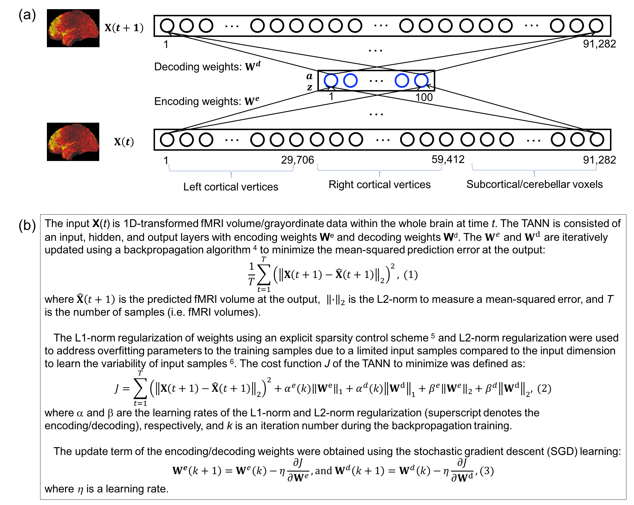
Figure 1 shows the (a) proposed TANN architecture and (b) training algorithm. The motor task fMRI runs of the Human Connectome Project (HCP) 2 were used to evaluate the TANN. All the input samples were repeatedly used 300 times (i.e. epochs) with a momentum strength of 0.5 3. The weights were updated in every 200 input samples using Eq. (3) of Fig. 1b. The η in Eq. (3) was initially 0.005 and gradually reduced to 0.00066 at 300 epochs; α in Eq. (2) was adaptively changed between 0 and 0.01 4,5; β in Eq. (2) was fixed to 10-5. The MATLAB codes implementing an autoencoding network (http://bspl.korea.ac.kr) were modified and multiple Linux machines (Intel i7; > 3GHz CPU; > 64GB RAM) were used to train the TANN model for each of two levels of the weight sparsity (i.e. Hoyer’s sparseness 6 of 0.5 and 0.7) and using smoothed or unsmoothed HCP fMRI volumes.
Once the TANN training was finished, the sign of the paired encoding/decoding features We(i) and Wd(i) associated with the ith hidden node was changed, so that the skewness of Wd(i) becomes positive 7. The highly task-specific Wd(i) were visualized using the “wb_view” tool and the time-series of the ith hidden node output corresponding to the input fMRI volume series were analyzed.
Results
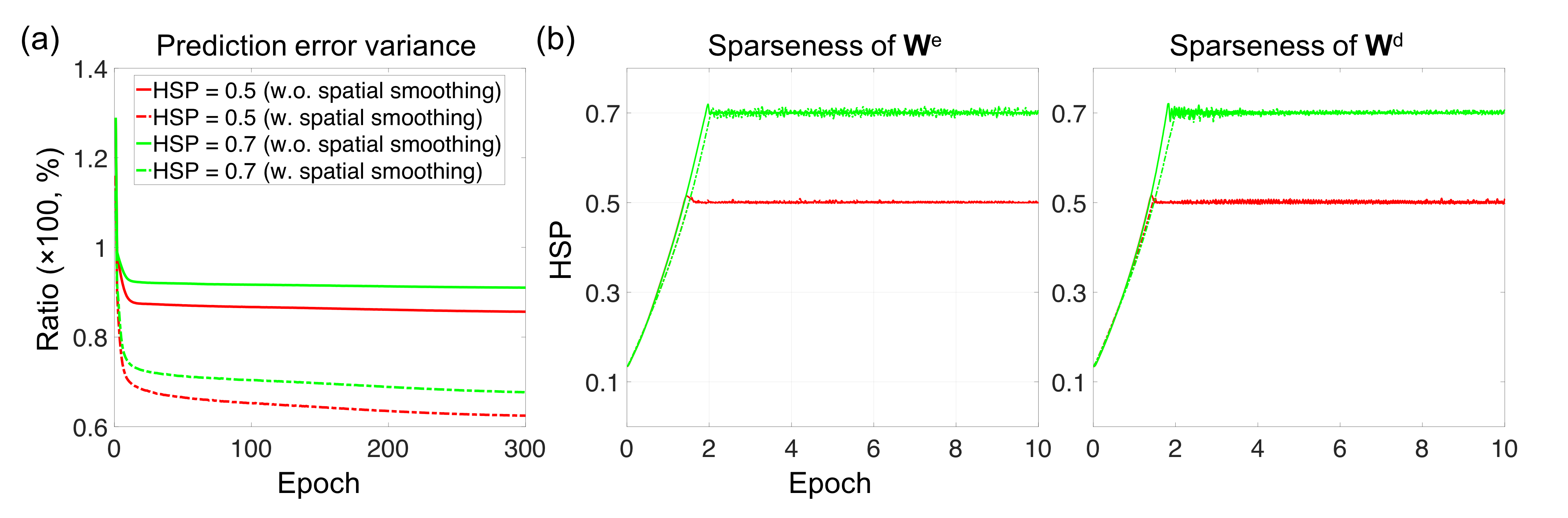
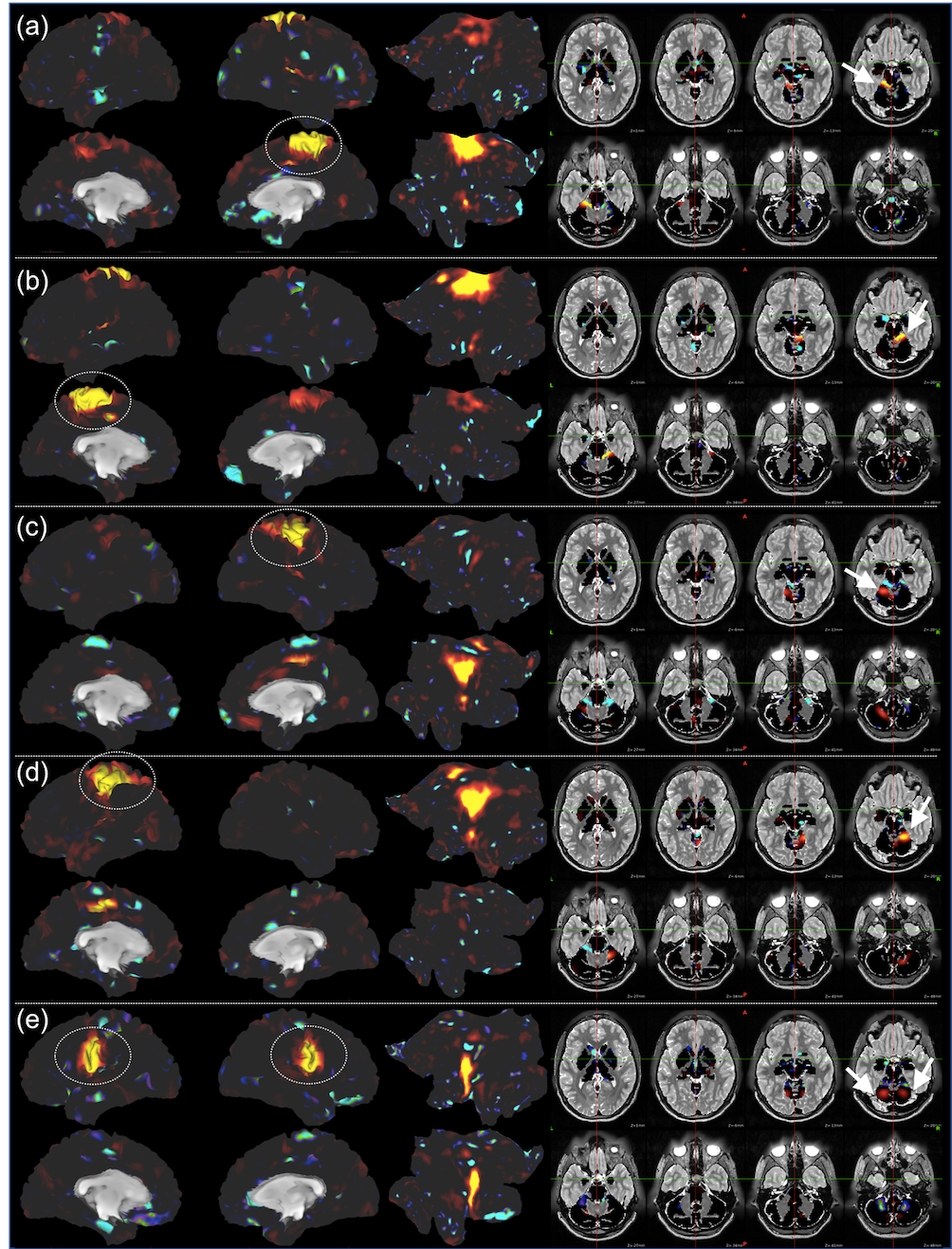
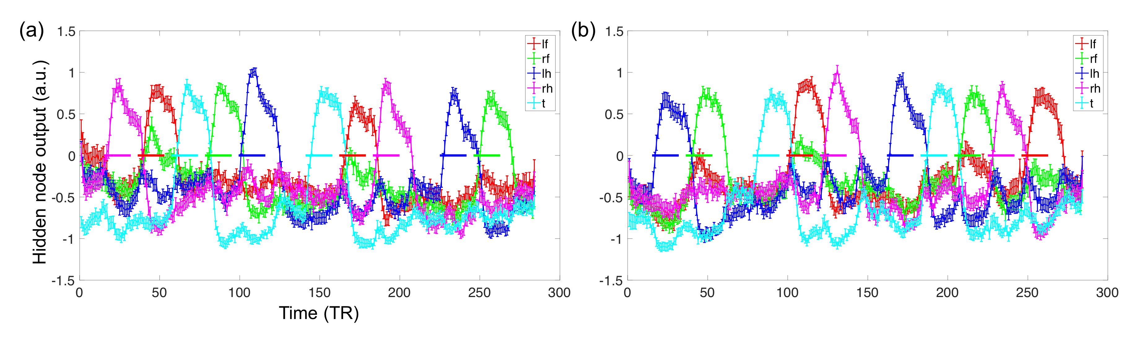
Fig. 2 shows the learning curves of the TANN training (took approximately 7 hours using the Linux computer: Intel i7-6700 3.4GHz CPU, 64GB RAM, and Ubuntu-16). The encoding/decoding weights from 82 hidden nodes out of 100 are localized within the brain area. The encoding/decoding features from the 18 remaining hidden nodes showed pseudo-randomly distributed spatial patterns which might be learnt to estimate thermal noises of the input fMRI volumes. Figs. 3 and 4 show the five most task-specific Wd(i) and the time-series of the corresponding ith hidden node output, respectively.
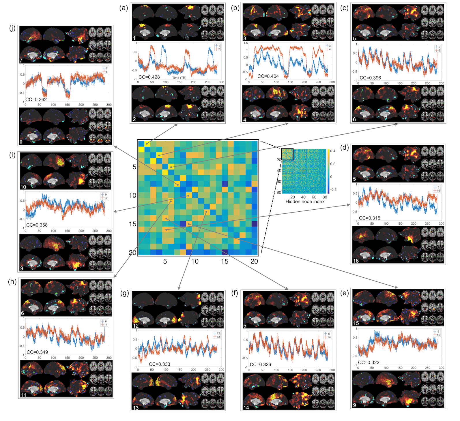
Fig. 5 shows the pairs of Wd(i), in which the output time-series of the corresponding hidden nodes are highly correlated. These pairs of hidden nodes are co-active along the task fMRI run and thus may reveal the functional dynamics associated with the task across the whole brain. For example, in (a), the foot-areas related hidden nodes showed the slightly greater ipsilateral activations from the left-toe than right-toe clenching task periods (i.e. at approximately 50 and 170 TRs). In (b), the visuo-motor (3) and parieto-motor (4) related hidden nodes were substantially active during the motor task periods, whereas these hidden nodes were quiet during the fixation/rest periods (i.e. 10, 140, 220, and 275 TRs). Interestingly, the hidden node (5) that represents the left superior-parietal/supramarginal, inferior temporal, inferior precentral, middle frontal areas are substantially co-active with multiple nodes that represent the bilateral precuneus (6 in c), left insula and its proximity (16 in d), and superior frontal and dorsal anterior cingulate (14 in f). In (g), the medial (12) and lateral (13) parts of the secondary visual cortices were separated into two hidden nodes and these networks are tightly co-active whenever visual cues were presented across the 13 blocks (i.e. the 10 motor and 3 fixation blocks).
Discussion
Our proposed computational neural network model revealed the human motor cortex dynamics in the HCP data. The highly task-specific foot, hand, and tongue networks were clearly identified from the decoding weights and the task-associated networks across the frontal, parietal, temporal, and visual areas were also clearly separated. The validity of these networks was supported by the temporal evolution of the associated hidden nodes. These functionally-parcellated networks from our TANN model and the associated time-series are currently examined such as comparing the results from alternative data-driven methods including ICA that would not reveal multiple components with highly correlated time-courses in the medial/lateral visual cortices (Fig. 5g).Conclusion
The proposed computational model appears to extract the underlying functional dynamics of each individual fMRI run without any task information. It is thus straightforward to apply this model to other sensory/motor/cognitive tasks and resting-state fMRI data.Acknowledgements
This work utilized the computational resources of the NIH HPC Biowulf cluster (http://hpc.nih.gov). This work was supported in part by Korea University Future Research Grant (KU-FRG).References
1. Hutchison RM, Womelsdorf T, Allen EA, et al. Dynamic functional connectivity: promise, issues, and interpretations. NeuroImage. 2013;80:360-378.
2. Glasser M, Coalson T, Robinson E, et al. A Multi-modal parcellation of human cerebral cortex. Nature. 2015.
3. LeCun YA, Bottou L, Orr GB, Müller K-R. Efficient backprop. Neural networks: Tricks of the trade: Springer; 2012:9-48.
4. Kim J, Calhoun VD, Shim E, Lee J-H. Deep neural network with weight sparsity control and pre-training extracts hierarchical features and enhances classification performance: Evidence from whole-brain resting-state functional connectivity patterns of schizophrenia. NeuroImage. 2016;124:127-146.
5. Jang H, Plis SM, Calhoun VD, Lee J-H. Task-specific feature extraction and classification of fMRI volumes using a deep neural network initialized with a deep belief network: Evaluation using sensorimotor tasks. NeuroImage. 2017;145(Pt B):314-328.
6. Hoyer PO. Non-negative matrix factorization with sparseness constraints. The Journal of Machine Learning Research. 2004;5:1457-1469.
7. Calhoun VD, Adali T, Pearlson GD, Pekar JJ. A method for making group inferences from functional MRI data using independent component analysis. Human brain mapping. 2001;14(3):140-151.
Figures