5609
The feasibility of absolute quantification for 31P MRS at 7T1OCMR, Department of Cardiovascular Medicine, University of Oxford, Oxford, United Kingdom
Synopsis
Calculation of in vivo concentrations requires knowledge of the B1 field. A common solution to this problem has been to use field maps measured in phantoms, but this becomes increasingly difficult at high field. The size of the effect of material and B0 field strength determining B1 in the liver using phosphorus (31P) phantoms was investigated at 1.5, 3, and 7T using CST simulations. The effect of concentration differences at 7T was demonstrated using 15 and 30mM phosphate phantoms. At 1.5T, using phosphate phantoms with concentrations between 5-40mM give an error of less than 3%. This increases to 10% at 3T, and 20-114% at 7T.
Purpose
The calculation of absolute concentrations in vivo requires a reference sample of known concentration1 and the signals from the scanned subject and the reference must be corrected for the difference in B1. A common solution to this problem has been to use field maps measured beforehand in phantoms2, 3. However, this becomes increasingly difficult at higher field strengths due to increased B1 inhomogeneity, making the material properties ever more important4. In this work, the impact of different material properties on 31P-MRS of the liver is investigated at 1.5, 3, and 7T to estimate the caution necessary when using phantoms for B1 inhomogeneity correction. B1+ fields were used, as they can be acquired in phantoms without prior knowledge of the full B1 field or use of adiabatic pulses.Methods
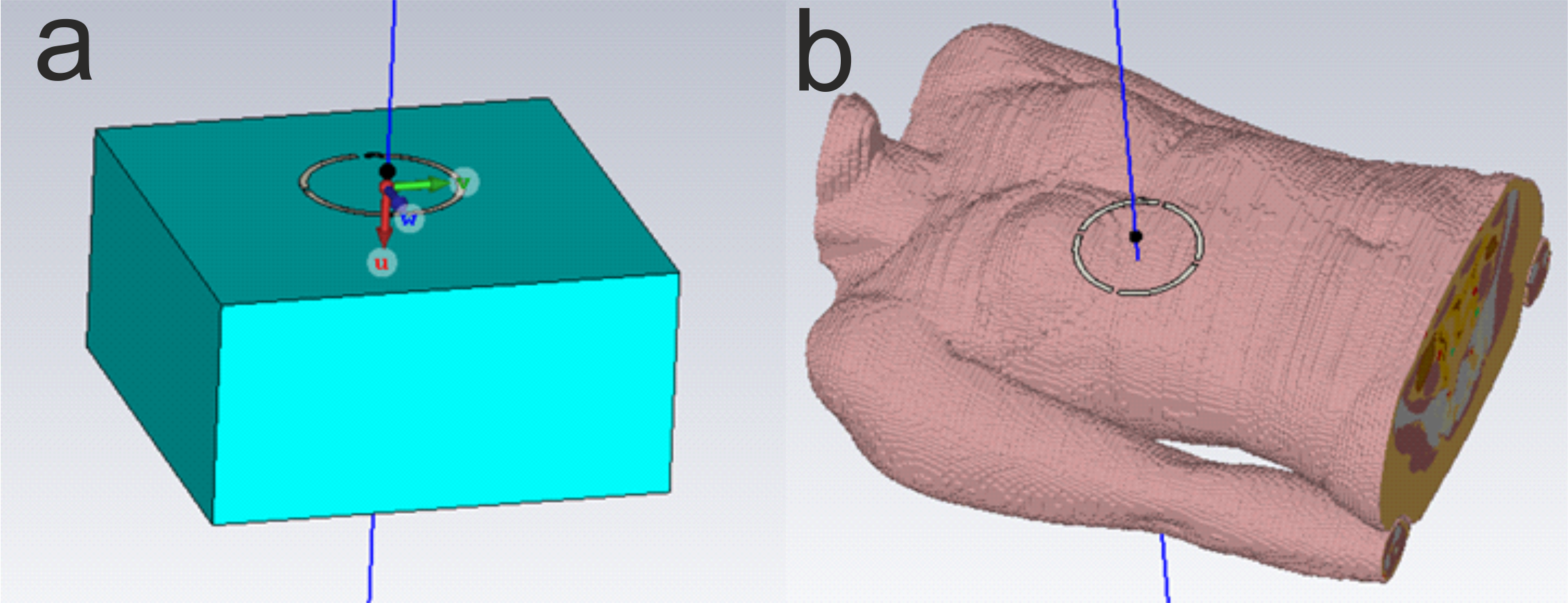
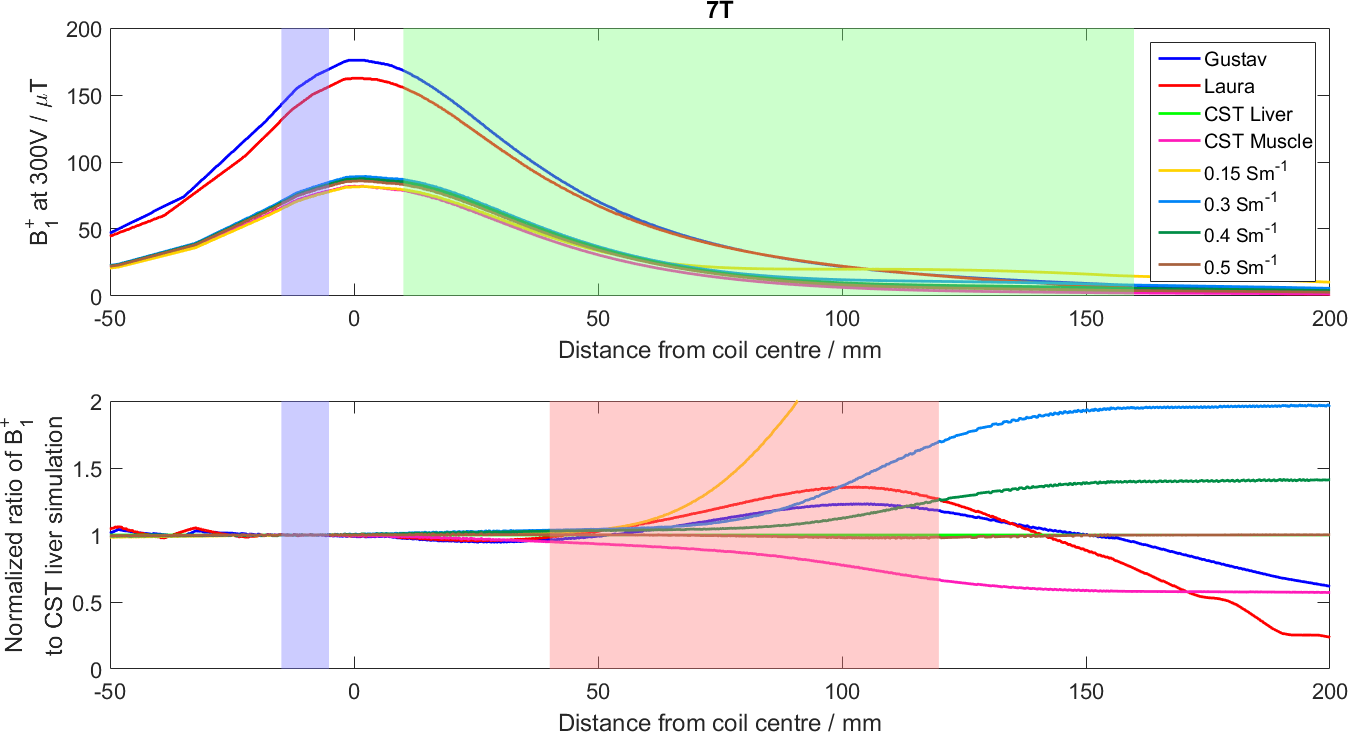
CST: CST Studio Suite 2016 (CST AG, Darmstadt, Germany) was used to simulate B1+ fields of a 10cm loop coil centred above a 300×300×150mm3 phantom and two voxel models, Laura and Gustav. The phantom materials used were the CST models for liver and muscle, and materials with conductivities of 0.02, 0.15, 0.5 and 2 Sm-1 to simulate various phosphate concentrations. The fields were simulated at 25.9, 49.9, and 120.3MHz. The coil was tuned and matched at each frequency, and the B1+ field was sampled along a line through the centre of the coil and phantom (see Figure 1). The B1+ profiles were normalized to a “reference fiducial” 10mm behind the face of the coil and averaged across the depth of the liver (see Figure 2).
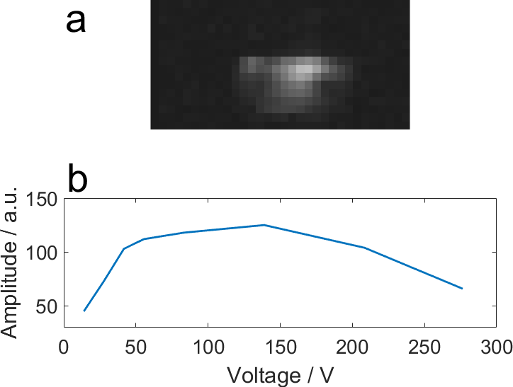
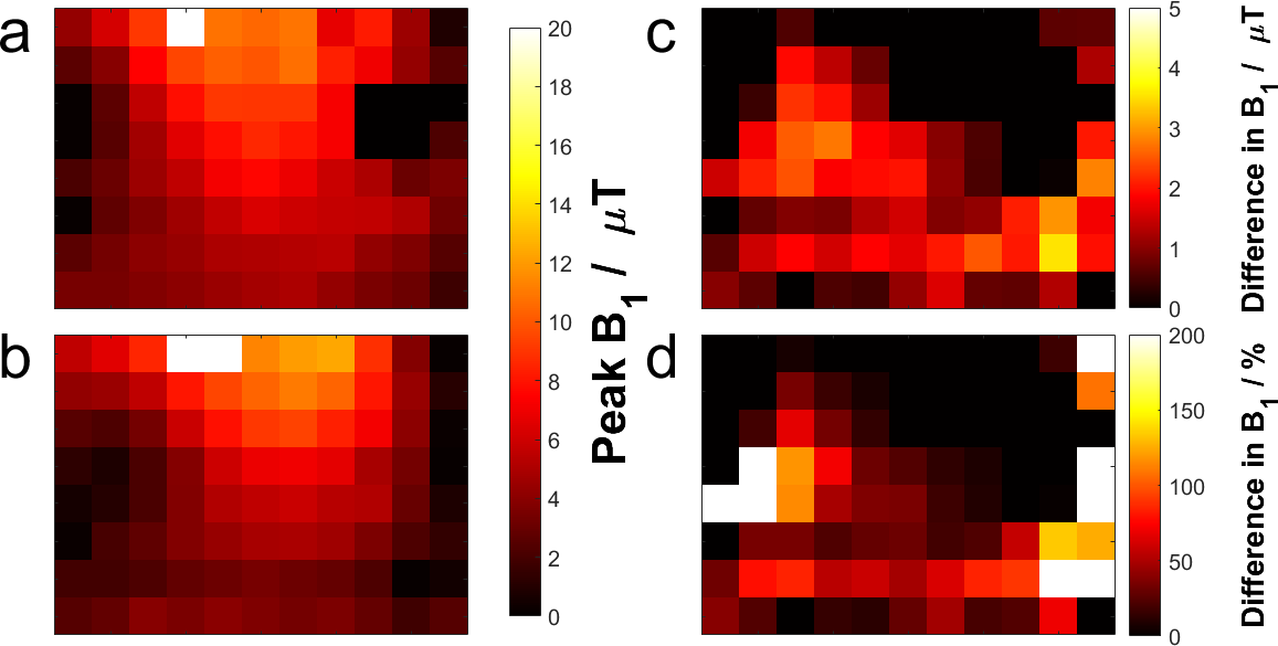
Phantom:Two K2HPO4(aq) phantoms (15mM and 30mM) with static conductivities (i.e. ω = 0) 0.30 and 0.54Sm-1, respectively5, were used. The conductivity is expected to be higher at 120.3MHz due to the Debye-Falkenhagen effect. All data were acquired on a Siemens Magnetom 7T system using a single 10cm diameter 1H loop and a custom-made 10cm 31P loop. Coil location and loading was calculated using a phenylphosphoric acid fiducials6. The T1 for each phantom was determined using non-localized inversion-recovery signals. Ten 31P 3D GRE images (32×16×18, 15.6×15.6×15mm3) were acquired with varying voltages. Transmit field maps were calculated by fitting saturation curves to each voxel, and simulating the B1+ required for the given flip angle.
Results and discussion
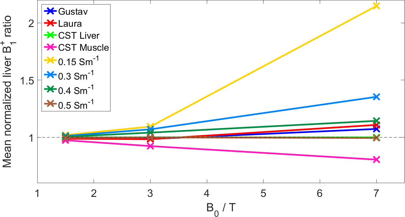
The CST B1+ ratios to the pure liver phantom are given for each material at several depths at 7T in Figure 2, and averaged over liver depths in Figure 3. They show that B0 field effects are important when considering the makeup of a phantom. The higher the field, the more closely the phantom must match in vivo tissue. At 1.5T, using a reference phantom with a conductivity of between 0.15 and 0.7Sm-1 would give an error of less than 3%. This increases to 10% at 3T, and 20-114% at 7T. These conductivities are equivalent to approximate K2HPO4(aq) concentrations of 5-40mM. The phantom field maps (see Figure 5) show that even concentrations as close as 15 and 30mM have significant differences in B1+. For less than 10% error at 7T, K2HPO4(aq) concentrations of 20-30mM should be used. At 3T, the difference between human voxel models is insignificant (<0.2%). At 7T, it becomes more important with differences of 3.5%. Simply matching the phantom conductivity to liver tissue would give 1.5% error at 3T and 10% error at 7T, but it is possible to more closely match the in vivo values with slightly lower conductivities. An example of the phosphate images in given in Figure 4. The amplitudes of a single pixel were plotted against voltage to show what was fitted. These results are a simplification of the problem that are meant to demonstrate the magnitude of the errors resulting from B0 field strength and phantom composition. This is shown by the field maps of the two phantoms at 7T, where the asymmetry due to conductivity can be seen. This effect twists the field in opposite directions for B1+ and B1-. However, as the magnitude of the change is expected to be the same, comparing B1+ can give an estimate of the error in B1- as well.Conclusion
In this study, the effect of phantom choice on B1 has been demonstrated in simulation at various field strengths. At 1.5T, a wide range of phantom conductivities (and therefore concentrations) can be used. At 3T, the errors are increased, but are still less than 10% for phosphate concentrations between 5-40mM. At 7T, even the differences between subjects start to be important, but if care is taken with phantom selection, errors can remain below 5%.Acknowledgements
Funded by a Sir Henry Dale Fellowship from the Wellcome Trust and the Royal Society (Grant Number 098436/Z/12/Z). LABP has a DPhil studentship from the Medical Research Council (UK).References
1. Bottomley PA. NMR Spectroscopy of the Human Heart. In: Harris RK, Wasylishen RE, editors. Encyclopaedia of Magnetic Resonance. Chichester: John Wiley; 2009.
2. Buchli R, et al. Magn Reson Med. 1994
3. Chmelik M, et al. Magn Reson Med. 2008
4. Vaidya MV, et al. Concepts Magn Reson Part B Magn Reson Eng. 2016
5. Pethybridge AD, et al. J Solution Chem. 2006
6. Rodgers CT, et al. Magn Reson Med. 2014
Figures