5519

Covariance Five Dimensional Echo Planar J-resolved Spectroscopic Imaging

Zohaib Iqbal¹ and M. Albert Thomas¹

¹Radiological Sciences, University of California - Los Angeles, Los Angeles, CA, United States

Synopsis

Chemical shift imaging is a very important method used to investigate several pathologies in vivo. A recent technological development incorporating an echo planar readout, a non-uniform sampling scheme, and an iterative, non-linear reconstruction is the five dimensional echo planar J-resolved spectroscopic imaging (5D EP-JRESI) method. While this technique is capable of obtaining 3 spatial and 2 spectral dimensions in vivo, the indirect spectral dimension has a low spectral resolution, which may hinder accurate metabolite quantitation. In this study, a novel approach using a covariance transformation after reconstruction is assessed and compared to the 5D EP-JRESI method.

Introduction

Chemical shift imaging (CSI) allows for noninvasive detection of several well-known biochemicals in the human brain and other regions of the body¹. By incorporating an echo planar readout, an echo planar spectroscopic imaging (EPSI) technique^2,3 is capable of greatly reducing scan time. Furthermore, a second spectral dimension can be incorporated into the acquisition of the EPSI sequence for better spectral disentanglement, giving rise to the echo planar J-resolved spectroscopic imaging method (EP-JRESI, or JRESI). Previously, this method has been accelerated using non-uniform sampling (NUS) and iterative, non-linear reconstruction to acquire 3 spatial and 2 spectral dimensions (5D JRESI) with eight-fold (8x) acceleration^4,5. However, the spectral resolution along the indirect dimension is very low for this type of acquisition. In this study, a novel method capable of improving spectral resolution using a covariance transformation is demonstrated and compared to the 5D JRESI method.

Methods

Acquisition and Reconstruction: The same acquisition and reconstruction methods detailed in a previous publication were used for this study⁵ to yield 5D data as $$$(x,y,z,F_2,F_1)$$$, where $$$x,y,z$$$ are the spatial dimensions and $$$F_2, F_1$$$ are the direct and indirect spectral dimensions, respectively. For all experiments, the following scan parameters were used: $$$(k_x,k_y,k_z,t_2,t_1)$$$ points = (16,16,8,256,64), direct spectral bandwidth = 1190Hz, indirect spectral bandwidth = 500Hz, and TE/TR = 30/1200ms.

A total of 10 in vivo healthy controls were scanned on a Siemens 3T Trio scanner (Siemens Healthcare, Erlangen, Germany). All volunteers were consented following IRB protocols. For in vivo acquisitions, the field of view (FOV) was chosen to produce a voxel resolution of 1.5x1.5x1.5cm$$$^3$$$. In addition to JRESI processing, the in vivo data were also reconstructed using the novel covariance transformation method as described below.

Covariance Transformation: The covariance transformation was applied to the maximum echo sampled⁶ spectra in the mixed spectral-temporal $$$A(F_2,t_1)$$$ domain following reconstruction to produce covariance JRESI (CovJRESI) data. The singular value decomposition (SVD) approach was utilized on a voxel-by-voxel basis in order to drastically decrease calculation time⁷ for calculating the covariance spectrum, $$$S$$$. A spectrum, $$$A(F_2,t_1)$$$, may be represented as the following using an SVD operation: $$$A = U\cdot W\cdot V^T$$$, where, $$$^T$$$ is the transpose operation. Afterwards, $$$S$$$ can readily be found: $$$S = U\cdot W \cdot U^T$$$. For the acquisition parameters above, the spectral resolution along the indirect dimension increases by a factor of 4 for CovJRESI data.

Simulations: A 5D virtual phantom was created using a 3D Shepp-Logan spatial profile. Each voxel contained a simulated 2D J-resolved spectrum with metabolites simulated using the GAMMA library⁸. Metabolite amplitudes were scaled to mimic typical in vivo gray matter concentrations: 7mM N-acetyl aspartate (NAA), 5mM Creatine (Cr), 2.5mM Phosphocholine (PCh), 10mM Glutamate (Glu), 3mM Glutamine (Gln), 4mM myo-Inositol (mI), and several other metabolites at 0.5-1mM. The virtual phantom was retrospectively sampled according to masks yielding four-fold (4x), 8x, twelve-fold (12x), and sixteen-fold (16x) acceleration, and these data were reconstructed as described previously⁵. Error metrics, such as root mean square error (RMSE) and normalized RMSE (nRMSE), were used to evaluate the performance of the reconstructed simulated data using both JRESI and CovJRESI for the total spectra and for individual metabolites: $$RMSE=\sqrt{\frac{\sum_{n}(y_f-y_r)^2}{n}}$$ $$$n$$$ is the number of points above the noise threshold for the given region, $$$y_f$$$ is the fully sampled, and $$$y_r$$$ is the reconstructed point. nRMSE was calculated by dividing RMSE by the average of the points.

Results

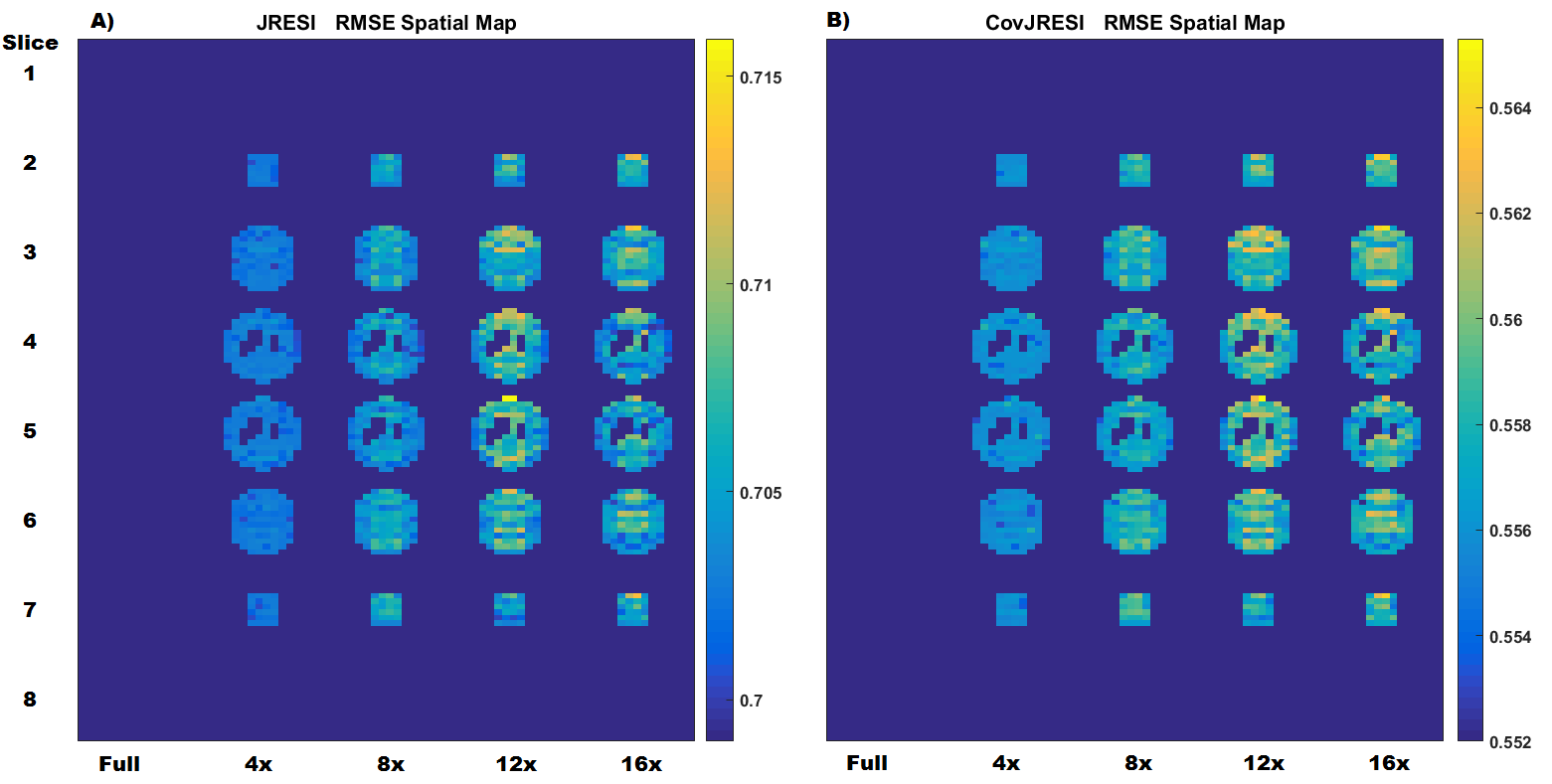
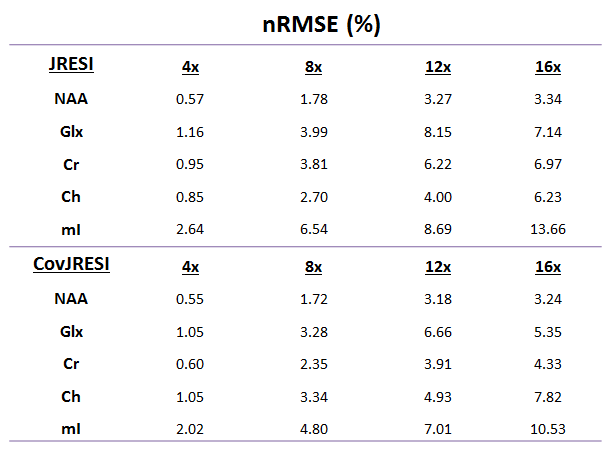
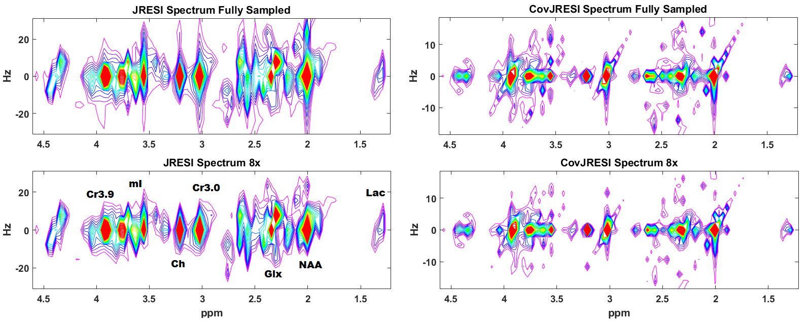
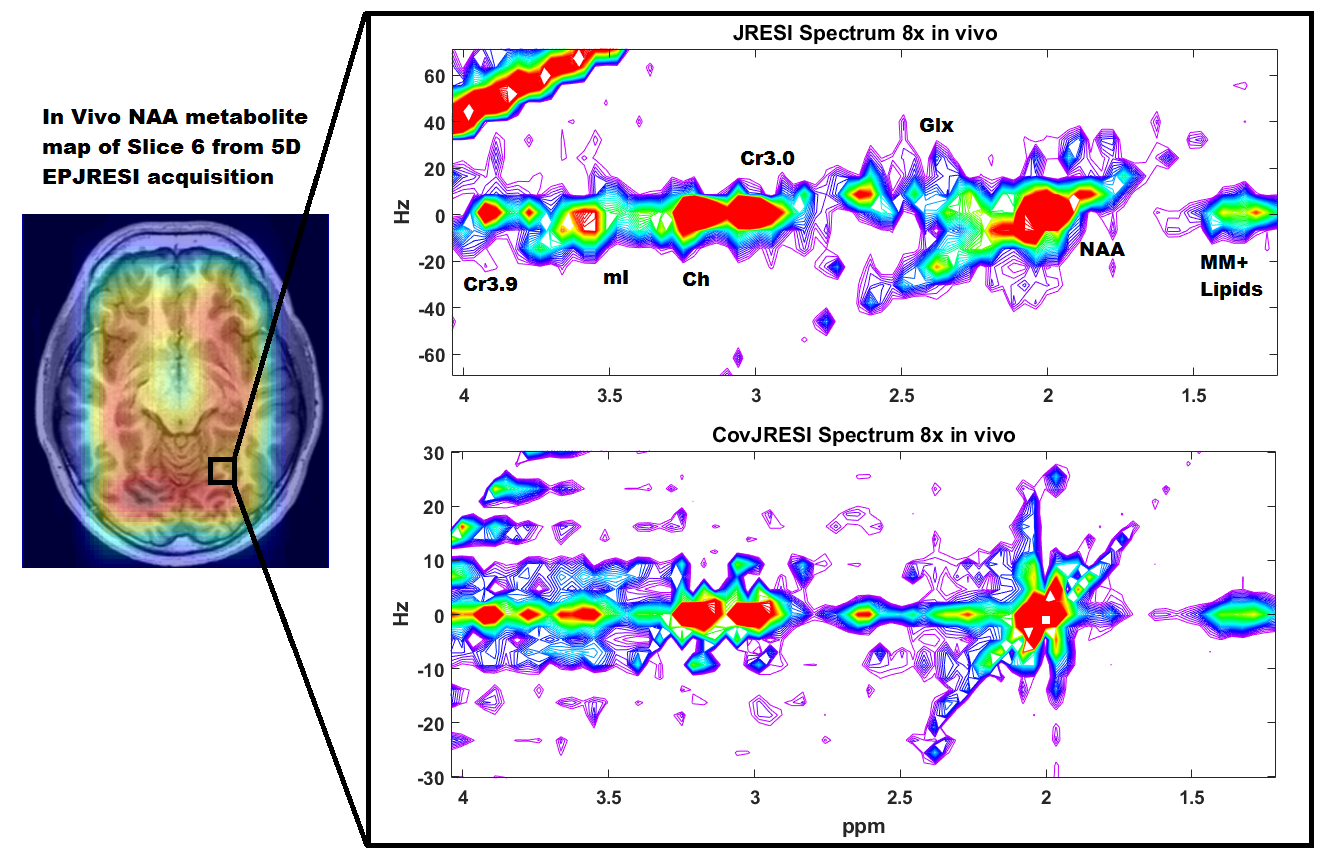
The total signal maps using the 5D EP-JRESI method on the virtual phantom can be seen in Figure 1. Figure 2 and Table 1 display the RMSE and metabolite specific nRMSE for both methods. Example spectra from the virtual phantom can be seen in Figure 3, and example in vivo spectra taken from a voxel of interest in the occipital region can be seen in Figure 4.

Discussion and Conclusions

A novel method for improving the spectral resolution of the 5D JRESI method is described. From Figure 2 and Table 1, it is clear that the CovJRESI method has smaller errors compared to the JRESI technique. This is due to the fact that signal is spread over more points, and seems to be especially true for J-resolved metabolites such as Glu, Gln, and mI. Spectra from both methods show good agreement when reconstructed after 8x acceleration both in the virtual phantom and in vivo. Future studies will focus on assessing whether CovJRESI offers better metabolite detection for Glu, Gln, mI, and others as a result of the increased spectral dispersion compared to the JRESI method.

Acknowledgements

The authors would like to acknowledge the UCLA Dissertation Year Fellowship, and the NIH R21 (NS080649-02) grant.

References

[1] Brown T, Kincaid B, Ugurbil K. NMR chemical shift imaging in three dimensions. Proceedings of the National Academy of Sciences 1982;79:3523-3526.

[2] Mansfield P. Spatial mapping of the chemical shift in NMR. Magnetic Resonance in Medicine 1984;1:370-386.

[3] Posse S, Tedeschi G, Risinger R, et. al. High Speed 1H Spectroscopic Imaging in Human Brain by Echo Planar Spatial-Spectral Encoding. Magnetic Resonance in Medicine 1995;33:34-40.

[4] Furuyama JK, Wilson NE, Burns BL, et. al. Application of compressed sensing to multidimensional spectroscopic imaging in human prostate. Magnetic Resonance in Medicine 2012;67:1499-1505.

[5] Wilson NE, Iqbal Z, Burns BL, et. al. Accelerated Five-dimensional echo planar J-resolved spectroscopic imaging: Implementation and pilot validation in human brain. Magnetic Resonance in Medicine 2016;75:42-51.

[6] Schulte RF, Lange T, Beck J, et. al. Improved two-dimensional J-resolved spectroscopy. NMR in Biomedicine 2006;19:264-270.

[7] Trbovic N, Smirnov S, Zhang F, Brüschweiler R. Covariance NMR spectroscopy by singular value decomposition. Journal of Magnetic Resonance 2004;171:277-283.

[8] Smith S, Levante T, Meier BH, Ernst RR. Computer simulations in magnetic resonance. An object-oriented programming approach. Journal of Magnetic Resonance, Series A 1994;106:75-105.

Figures

Figure 1. The 3D Shepp Logan spatial profile for the fully sampled 5D JRESI experiment is shown, alongside the spatial profiles for the non-uniformly sampled and reconstructed data using 4x, 8x, 12x, and 16x acceleration. The spatial profiles are displaying the total signal projected from the 1 - 4.3ppm region for the virtual phantoms. As expected, when acceleration increases, reconstruction quality diminishes. However, even at 16x acceleration, the spatial profile for the virtual phantom is still recognizable.

Figure 2. The root mean square error (RMSE) maps for all of the acceleration factors are displayed for both the JRESI method (left) and the CovJRESI method (right). From the scales, it is apparent that the CovJRESI has less overall error when compared to the fully sampled data. This is due to the fact that using the covariance transformation helps further spread the signal along the indirect spectral dimension, which increases $$$n$$$ in the RMSE calculation.

Table 1. All of the normalized root mean square error (nRMSE) values are tabulated for each metabolite using 60 voxels from the virtual phantom. The following metabolite regions were used to calculate nRMSE: NAA (1.9 - 2.1ppm), Glu + Gln (Glx, 2.2 - 2.5ppm), Cr (2.9 - 3.1ppm), PCh (3.1 - 3.3ppm), and mI (3.4 - 3.6ppm). All nRMSE values were calculated by using ±20Hz in the indirect spectral dimension. J-resolved metabolites such as Glx and mI show much more error as the acceleration factors increase.

Figure 3. Example spectra from both the JRESI (left) and CovJRESI (right) methods are shown from a central voxel in the 3D Shepp-Logan phantom. Also, the spectra reconstructed after 8x acceleration are shown below the fully sampled spectra. Qualitatively, both the fully sampled and 8x spectra look very similar for both the JRESI and CovJRESI method, implying that the reconstruction was accurate. Subtle differences, however, yield the RMSE and nRMSE results seen in Figure 2 and Table 1.

Figure 4. The axial MRI with an NAA map overlay is shown from a 20 year old, healthy volunteer. The NAA map was produced by taking the integral of NAA in each voxel and projecting it spatially for this slice. A spectrum from both the JRESI and CovJRESI methods can be seen. The major metabolites, NAA, Glu + Gln (Glx), Creatine 3.0 (Cr3.0), PCh (or Ch), mI, and Creatine 3.9 (Cr3.9) are shown. Also, macromolecule (MM) and lipid signal can be seen in the spectra. More spectral spread can be seen in the CovJRESI spectrum.

Proc. Intl. Soc. Mag. Reson. Med. 25 (2017)

5519