Synopsis

Estimating a set of coil sensitivity maps that is consistent with the low-resolution SENSE model is challenging in SENSE spectroscopic imaging. Recently, ESPIRiT, an autocalibrating approach to estimate sensitivity maps for MR imaging, that combines both advantages of SENSE and GRAPPA has been developed. In this work, we propose a spectroscopic extension of ESPIRiT, referred to as S-ESPIRiT, to estimate sensitivity maps from Cartesian 2D spectroscopic k-space data. The proposed method was demonstrated using 2D spectroscopic imaging data of a brain metabolite phantom acquired with a semi-LASER pulse sequence and a 32-channel receive head coil on a 7T MRI scanner.

Introduction

Estimating an accurate set of coil sensitivity maps that is consistent with the low-resolution SENSE model¹ (a non-Dirac point spread function) is challenging in SENSE spectroscopic imaging^2,3. Recently, ESPIRiT⁴, an autocalibrating approach to estimate sensitivity maps for MR imaging, has been developed. In this work, we propose a spectroscopic extension of ESPIRiT, referred to as S-ESPIRiT, to estimate sensitivity maps from Cartesian 2D spectroscopic k-space data.

Methods

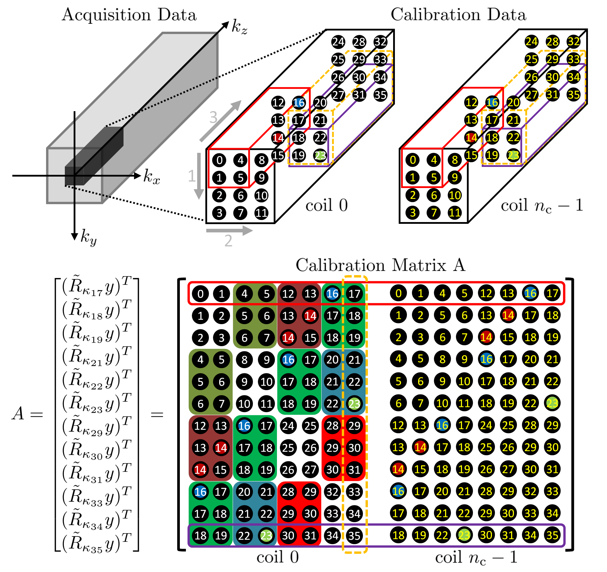
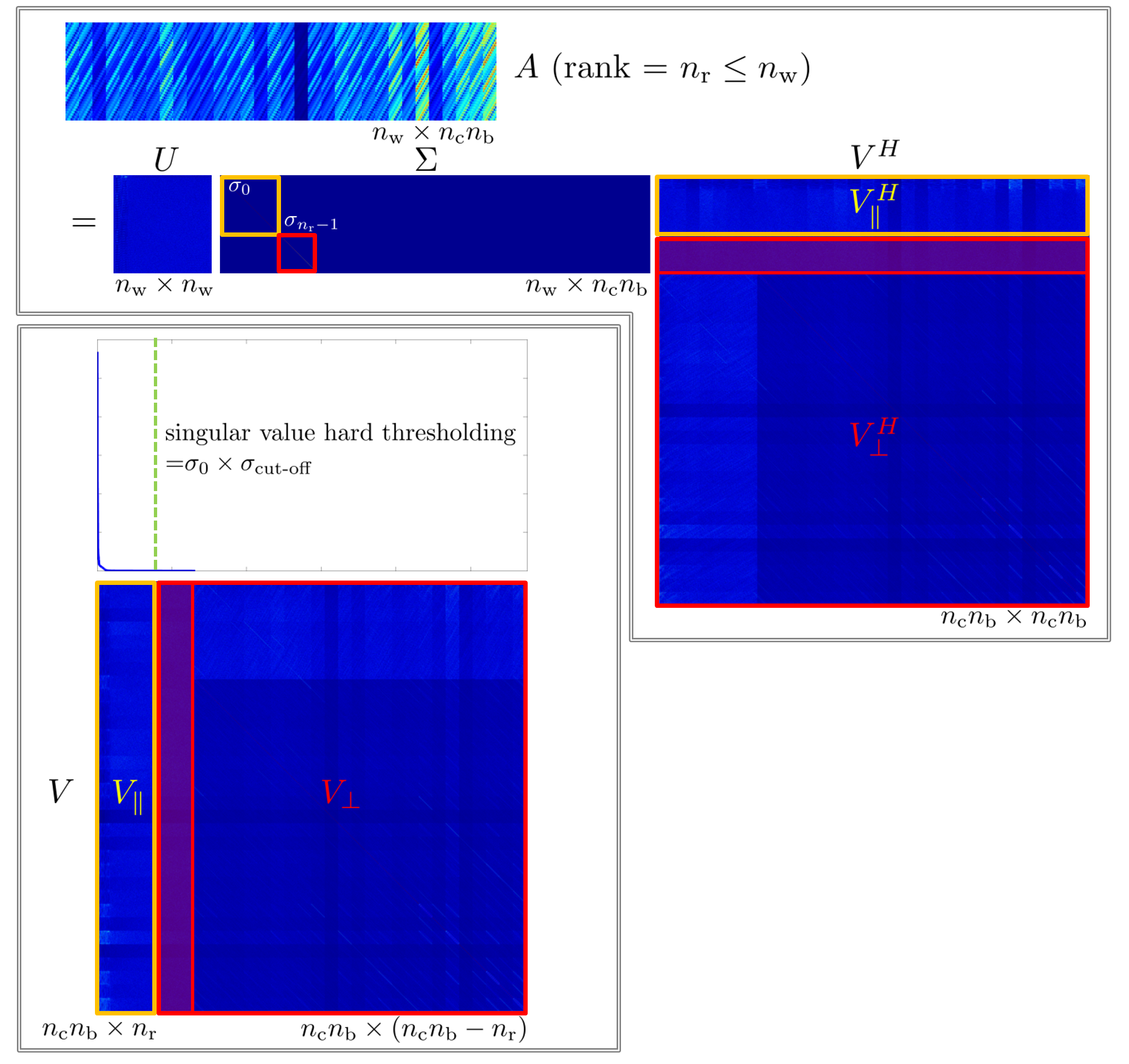
We consider two-dimensional (2D) Cartesian parallel spectroscopic imaging. Let $$$n_k$$$ and $$$n_t$$$ denote the numbers of k-space positions in spatial dimensions and spectral dimension in a fully sampled Cartesian grid, respectively. Let $$$R_\kappa:\mathbb{R}^{n_k n_t}\to\mathbb{R}^{n_b}$$$ be the sampling operator that first chooses a block of k-space samples out of a single-channel Cartesian grid, where a block is of size $$$n_{k_y}^b\times n_{k_x}^b\times n_{t}^b$$$ and centered at position $$$\kappa$$$, and then vectorize the block of k-space samples into a column vector of size $$$n_b$$$. With the Kronecker product $$$\otimes$$$, we express multichannel sampling operator $$$\tilde{R}_\kappa:\mathbb{R}^{n_c n_k n_t}\to\mathbb{R}^{n_c n_b}$$$ as $$$\tilde{R}_{\kappa}=Id_{n_c}\otimes R_{\kappa}$$$. Let the size of calibration data be $$$n_{k_y}^{AC}\times n_{k_x}^{AC}\times n_{t}^{AC}$$$. Then, the number of sliding windows in a calibration region is given by $$$n_w=(n_{k_y}^{AC}-n_{k_y}^{b}+1)(n_{k_x}^{AC}-n_{k_x}^{b}+1)(n_{t}^{AC}-n_{t}^{b}+1)$$$. Following the ESPIRiT formalism for MR imaging⁴, a calibration matrix $$$A\in\mathbb{C}^{n_w\times n_c n_b}$$$ for 2D spectroscopic imaging is defined. Figure 1 shows a detailed description of constructing a calibration matrix A for 2D spectroscopic imaging. The singular value decomposition (SVD) of a calibration matrix gives $$$A = U\Sigma V^H $$$, where $$$\Sigma\in\mathbb{C}^{n_w\times n_c n_b}$$$ is the matrix of sigular values, and $$$V\in\mathbb{R}^{n_c n_b\times n_c n_b}$$$ is the matrix of right singular vectors. $$$V$$$ can be decomposed into $$$V_{\|}\in\mathbb{C}^{n_c n_b\times n_r}$$$ that is a basis for the row space of A and $$$V_{\perp}$$$ that is a basis for the null space of A. Figure 2 illustrates an example of the singular value decomposition of a calibration matrix for spectroscopic imaging k-space data. Since $$$V_{\|}$$$ is a basis for the overlapping blocks of k-space in calibration data, $$$V_{\|}$$$ can be a good basis for any blocks of k-space, namely, a projection of a block $$$\tilde{R}_{\kappa}y$$$ onto $$$V_{\|}$$$ should be $$$V_{\|}V_{\|}^H\tilde{R}_{\kappa}y=\tilde{R}_{\kappa}y$$$. Therefore, this leads to the ESPIRIT conditions for the multichannel k-space data $$$x$$$⁴:\begin{equation}\underbrace{\frac{1}{n_b}\sum_{\kappa=0}^{n_k n_t-1} \tilde{R}_{\kappa}^H V_{\|}V_{\|}^H\tilde{R}_{\kappa}}_{\mathcal{W}}x=x.\end{equation} Using the Cartesian SENSE model¹, multichannel Cartesian k-space data $$$x\in\mathbb{C}^{n_k n_t}$$$ is related to a 2D spectroscopic image $$$m\in\mathbb{C}^{n_k n_t}$$$ by $$$x = \tilde{F}\tilde{S}m$$$, where $$$\tilde{F}:\mathbb{C}^{n_c n_k n_t}\to\mathbb{C}^{n_c n_k n_t}$$$ is the Fourier operator that performs a coil-wise 3D DFT, and $$$\tilde{S}:\mathbb{C}^{n_k n_t}\to\mathbb{C}^{n_c n_k n_t}$$$ is the sensitivity operator that generates full-FOV coil images. Substituting for $$$x$$$ and multiplying $$$\tilde{F}^{-1}$$$ on both sides of the equation yields an eigenvalue problem (with eigenvalue "=1") for the coil images:$$\mathcal{G}\tilde{S}m=\tilde{S}m,$$ where $$$\mathcal{G}=\tilde{F}\mathcal{W}\tilde{F}^{-1}$$$. To simplify the equation, we explicitly express each term in $$$\mathcal{G}$$$ and $$$V_{\|}$$$ in block form where each kernel is broken into per-channel-kernels $$$v_{r}=[v_{r,0},v_{r,1},v_{r,n_c-1}]^T$$$:\begin{align}\mathcal{G} &=\left(Id_{n_c}\otimes H_{n_k n_t}\right)\left(\frac{1}{n_b}\sum_{\kappa=0}^{n_k n_t-1}(Id_{n_c}\otimes R_{\kappa}^H)V_{\|}V_{\|}^H (Id_{n_c}\otimes R_{\kappa})\right)\left(Id_{n_c}\otimes H_{n_k n_t}^H\right)\\&=\frac{1}{n_b}\sum_{\kappa=0}^{n_k n_t-1}\left[\left(Id_{n_c}\otimes H_{n_k n_t}R_{\kappa}^H\right)V_{\|}V_{\|}^H\left(Id_{n_c}\otimes R_{\kappa}H_{n_k n_t}^H\right)\right]\\&=\frac{1}{n_b}\sum_{\kappa=0}^{n_k n_t-1}g_{\kappa}g_{\kappa}^H,\end{align}where\begin{align}g_{\kappa}=\left[\begin{array}{@{}c:c:c@{}}g_{\kappa,(0,0)}=H_{n_k n_t}R_{\kappa}^H v_{0,0}&g_{\kappa,(1,0)}&g_{\kappa,(n_r-1,0)}\\ \hdashline g_{\kappa,(0,1)}&g_{\kappa,(1,1)}&g_{\kappa,(n_r-1,1)}\\ \hdashline g_{\kappa,(0,n_c-1)}&g_{\kappa,(1,n_c-1)}&g_{\kappa,(n_r-1,n_c-1)}\end{array}\right], \mathrm{and} \, \, g_{\kappa,(r,\gamma)} =\left[\begin{array}{c} g_{\kappa,(r,\gamma)}(\vec{r}_{0}) \\ g_{\kappa,(r,\gamma)}(\vec{r}_{1}) \\ g_{\kappa,(r,\gamma)}(\vec{r}_{n_k n_t-1}) \end{array}\right] \in \mathbb{C}^{n_k n_t}.\end{align}

By the Fourier shift theorem in k-space, if $$$g_{c,(r,\gamma)}=H_{n_k n_t}R_{c}^H v_{(r,\gamma)}$$$, where $$$c$$$ is the voxel index for zero spatial coordinates in image space, then $$$g_{\kappa,(r,\gamma)}= \Phi_{\kappa} g_{c,(r,\gamma)}$$$, where $$$\Phi_{\kappa} \in \mathbb{C}^{n_k n_t \times n_k n_t}$$$ is diagonal with $$$\Phi_{\kappa}(\rho,\rho) = e^{+j \vec{\omega}_{\kappa} \cdot \vec{r}_{\rho}}$$$.

A further simplification leads to a block diagonal structure in $$$\mathcal{G}$$$: \begin{equation} \mathcal{G}=\left[\begin{array}{@{}c:c:c@{}} \mathcal{D}(G_{0,0}) & \mathcal{D}(G_{1,0}) & \mathcal{D}(G_{n_r-1,0}) \\ \hdashline \mathcal{D}(G_{0,1}) & \mathcal{D}(G_{1,1}) & \mathcal{D}(G_{n_r-1,1}) \\ \hdashline \mathcal{D}(G_{0,n_c-1}) & \mathcal{D}(G_{1,n_c-1}) & \mathcal{D}(G_{n_r-1,n_c-1}) \\ \end{array}\right], \end{equation} where $$$\mathcal{D}(\cdot)$$$ is an operator that selects only diagonal terms and $$$G_{\gamma, \gamma'}(\rho,\rho') = \Sigma_{r=0}^{n_r-1} g_{c,(r,\gamma)}(\vec{r}_{\rho}) g_{c,(r,\gamma')}^H (\vec{r}_{\rho'})$$$.

This diagonal structure decouples voxels and leads to individual eigenvalue decomposition at voxel with non-zero signal value:\begin{equation} \left[\begin{array}{@{}ccc@{}} \mathcal{G}_{0,0}(\vec{r}_{\rho}) & \mathcal{G}_{0,1}(\vec{r}_{\rho}) & \mathcal{G}_{0,n_c-1}(\vec{r}_{\rho}) \\ \mathcal{G}_{1,0}(\vec{r}_{\rho}) & \mathcal{G}_{1,1}(\vec{r}_{\rho}) & \mathcal{G}_{1,n_c-1}(\vec{r}_{\rho}) \\ \mathcal{G}_{n_c-1,0}(\vec{r}_{\rho}) & \mathcal{G}_{n_c-1,1}(\vec{r}_{\rho}) & \mathcal{G}_{n_c-1,n_c-1}(\vec{r}_{\rho}) \\ \end{array}\right] \left[\begin{array}{@{}c@{}} S_0(\vec{r}_{\rho}) \\ S_1(\vec{r}_{\rho}) \\ S_{n_c-1}(\vec{r}_{\rho}) \end{array}\right] m(\vec{r}_{\rho})=\left[\begin{array}{@{}c@{}} S_0(\vec{r}_{\rho}) \\ S_1(\vec{r}_{\rho}) \\ S_{n_c-1}(\vec{r}_{\rho}) \end{array}\right] m(\vec{r}_{\rho}).\end{equation}

Results

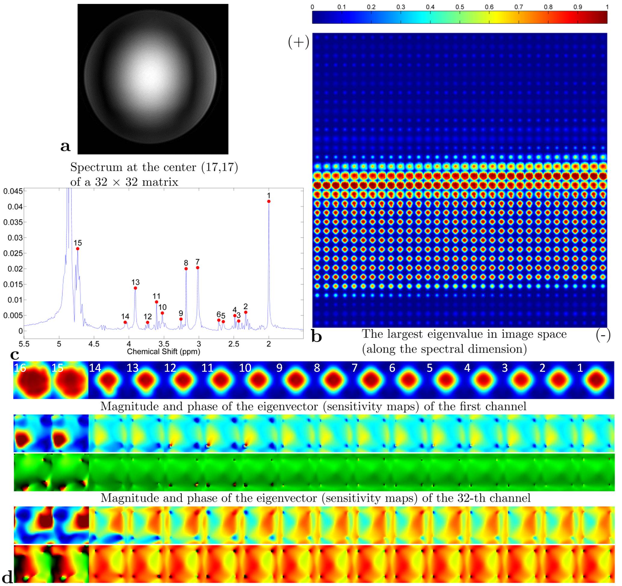
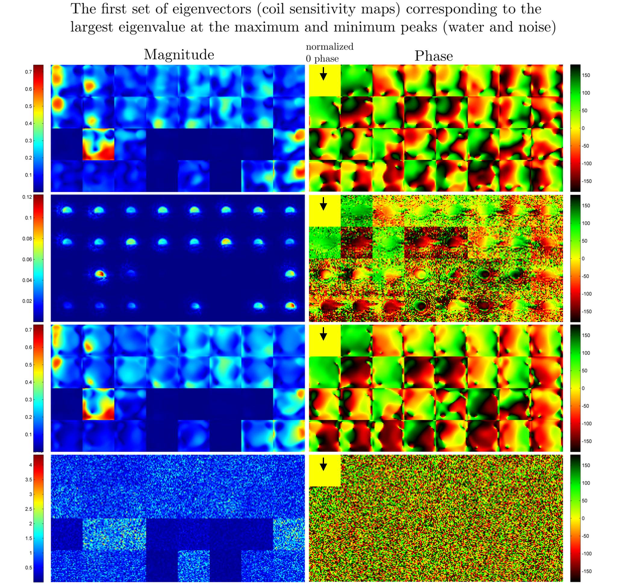
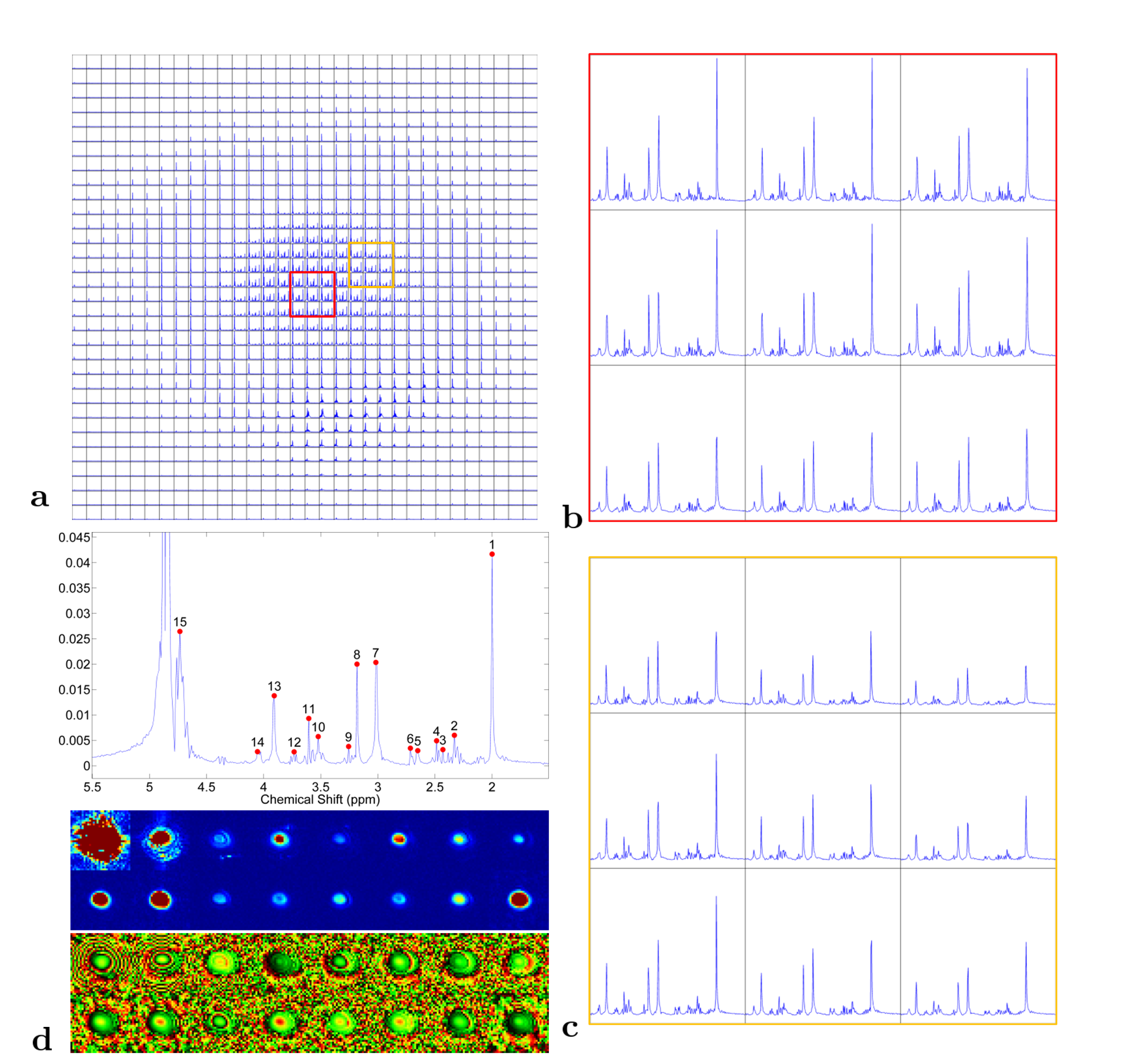
A semi-LASER pulse sequence⁵ was used to acquire 2D spectroscopic imaging data of a brain metabolite phantom with a 32-channel receive head coil on a 7T human MRI scanner. Figure 3-5 show the largest eigenvalue maps, sensitivity maps (the first set of eigenvectors), and SENSE-reconstructed spectra using the sensitivity maps estimated by S-ESPIRiT, respectively. A detailed description for each result is provided in the figure caption.

Conclusion

This work presents a novel autocalibrating method to estimate coil sensitivity maps from Cartesian 2D spectroscopic data. The proposed method was demonstrated using a phantom data set, showing promising results. A further study using human datasets is required to validate the robustness of S-ESPIRiT.

Acknowledgements

This research was supported in part by the Danish Agency for Science, Technology and Innovation via grant International Network Programme and by KBSI grant T36418 (N.L. and G.C.).

References

1. Pruessmann KP, Weiger M, Scheidegger MB, Boesiger P. SENSE: sensitivity encoding for fast MRI. Magn Reson Med 1999;42:952–962.

2. Zhao X, Prost RW, Li SJ. Reduction of artifacts by optimization of the sensitivity map in sensitivity-encoded spectroscopic imaging. Magn Reson Med 2005;53:30-34.

3. Dydak U, Weiger M, Pruessmann KP, Meier D, Boesiger P. Sensitivity-encoded spectroscopic imaging. Magn Reson Med 2001;46:713–722.

4. Uecker M, Lai P, Murphy MJ, Virtue P, Elad M, Pauly JM, Vasanawala SS, Lustig M. ESPIRiT—an eigenvalue approach to autocalibrating parallel MRI: where SENSE meets GRAPPA. Magn Reson Med 2014;71:990–1001.

5. Boer VO, van Lier AL, Hoogduin JM, Wijnen JP, Luijten PR, Klomp DW. 7-T (1) H MRS with adiabatic refocusing at short TE using radiofrequency focusing with a dual-channel volume transmit coil. NMR Biomed 2011;24:1038–1046.