5483

Impact of time sample selection and model function design on the quantification of fatty acid composition: in vitro and in vivo studies.

Angeline Nemeth¹, Hélène Ratiney¹, Benjamin Leporq¹, Amandine Coum^2,3, Giulio Gambarota^2,3, Kevin Seyssel⁴, Bérénice Segrestin⁵, Pierre-Jean Valette⁶, Martine Laville⁵, and Olivier Beuf¹

¹Univ. Lyon, INSA‐Lyon, Université Claude Bernard Lyon 1, UJM-Saint Etienne, CNRS, Inserm, CREATIS UMR 5220, U1206, F69621, Lyon, France, ²INSERM, UMR 1099, Rennes, France, ³Univ Rennes 1, LTSI, Rennes, France, ⁴Department of Physiology, Faculty of Biology and Medicine, University of Lausanne, Lausanne, Switzerland, ⁵Centre de Recherche en Nutrition Humaine Rhône-Alpes (CRNH-RA), Centre Hospitalier Lyon Sud, Pierre-Bénite, Lyon, France, ⁶Hospices Civils de Lyon, Département d'imagerie digestive, CHU Edouard Herriot, Lyon, France

Synopsis

Interest in the follow-up of fatty acid composition(saturated, polyunsaturated and monounsaturated fatty acid) in the body is growing. Quantitative MR spectroscopy can give access to this fat composition. Today, several quantification methods are used (e.g LCModel, AMARES). However the statistical outcome issued from a quantitative analysis of the lipid signal can be greatly influenced by the used quantification method. We analyze 1) the impact of the time sample selection and design of the model function on the parameter identifiability 2) the quantification results obtained with different quantification models on acquisitions performed in vitro (oils) and in vivo (subcutaneous adipose tissue).

Purpose

Interest in the fat quantification has grown in recent years. In particular, the nutrition studies are interested in the variation of fatty acid composition in the body: saturated fatty acid (SFA), polyunsaturated (PUFA) and monounsaturated (MUFA). Magnetic resonance spectroscopy (MRS) is a quantitative technique that gives access to this fat composition. At this time, several quantification methods, primarily developed for brain MRS analysis, are used (e.g LCModel, AMARES). However, it has been recently described that, in the case of lipid signal, the statistical outcome issued from a quantitative analysis can be greatly influenced by the used quantification method¹.

In the present work, we investigate the particular case of lipid quantification in adipose tissue; for which the lipid components are predominant and we study the impact of the time sample selection and design of the model function on the parameter identifiability (given by the condition number of the Jacobian Matrix²) and on the parameter relative Cramer Rao Lower Bound (CRLB). These two criteria give insight about the ability of the parameter estimation to provide precise inference. We then analyze the quantification results obtained with different quantification models- adding results from the reference LCModel method- on in vitro oil and in vivo subcutaneous adipose tissue (AT) acquisitions.

Materials and methods

In vitro MRS was performed on a preclinical 4.7T BioSpec Bruker system, a PRESS sequence was used with TR = 5000 ms, TE = 7.89 ms, VOI of 4×4×4 mm3, 32 signal averages; on 10 commercial oils.

In vivo MRS was carried out on Philips Ingenia 3T system the STEAM sequence was used with TR= 3000ms, TE= 14ms, VOI of 20×20×20 mm3, 4 signal averages and 1024 data points. On five subjects, an MR spectrum was acquired twice (for test retest) in the abdominal subcutaneous AT using respiratory triggering.

Most of the MRS quantification methods are based on a model function to be adjusted to the acquired data. When fitting in the time domain the time sample used in the fitting procedure can be selected.

Studied Model functions.

The first studied model function is inspired from a quantification method applied on multi-gradient echo imaging³ (Eq.1). $$Eq.1:f(t)=\left(A_w*n_{water}+A_f*\sum_{k=1}^8n_k(ndb,nmidb)*e^{2i{\pi}f_kt}\right)e^{-\frac{t}{T2^*}}$$ The second model is based on a Voigt Model⁴ (Eq.2) close to AMARES signal description.$$Eq.2:f(t)=e^{i\phi_0}*\sum_{k=1}^9c_ke^{\alpha_kt+\left(\beta_kt\right)^2+2i{\pi}f_kt}$$

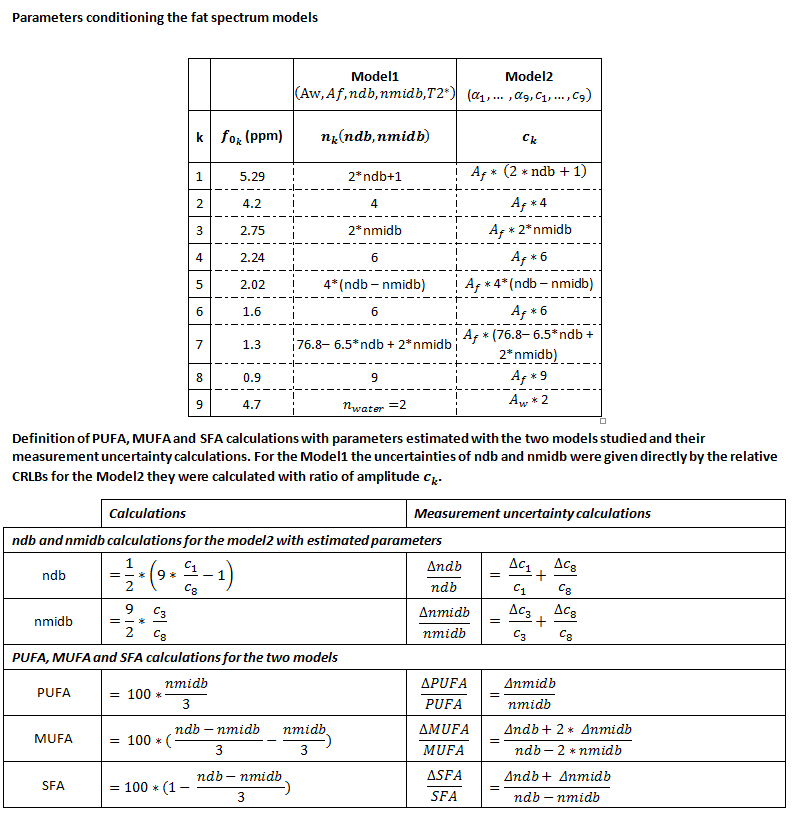
In the case of the lipids, the relative amplitudes of the peaks are linked (see Table1). These relations can be introduced in the model (Model1) or deduced from the fitted component amplitude (Model2).

Undersampling of temporal signal within the fitting procedure was tested with $$$t=n*t_e$$$ with $$$t_e=\frac{1}{2*(4.7-1.3)*B_0*\frac{\gamma}{2\pi}}$$$, the results presented below were for n=32.

Theoretical model comparison

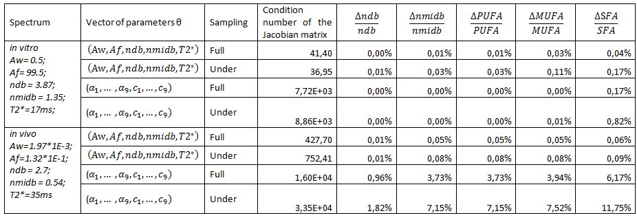
For each model function and each case (oils and in vivo), some realistic parameter values were used and the condition number of the Jacobian matrix (cond-J), and the parameter uncertainty, $$$\frac{\triangle\theta}{\theta}$$$, as the relative the CRLBs, were computed ($$$\frac{\triangle\theta}{\theta}=\sigma_0*\frac{\sqrt{F(\theta)^{-1}}}{\theta}$$$ where $$$\theta=\left\{ndb,nmidb,c_1,c_3,c_8\right\}$$$, $$$F^{-1}=\left[J^T.J\right]^{-1}$$$ the inverse Fisher matrix and $$$\sigma_0$$$ standard deviation of noise, for PUFA, MUFA and SFA the calculation is detailed in table1.

Five estimated parameters $$$(A_w,A_f,ndb,nmidb,T2^*)$$$ for Model1 and 2*9 estimated parameters $$$(\alpha_1,...,\alpha_9,c_1,...,c_9)$$$ for Model2 were considered. Indeed, to be sure that the two models describe mathematically the same signal we used for Model2: $$${\phi_0}=0$$$, $$${\alpha_k}=-\frac{1}{T2^*}$$$, $$$ {\beta_k}=0$$$, $$$c_k=A_f*n_k(ndb,nmidb)$$$ for $$$k=\left\{1,...,8\right\}$$$, $$$c_9=A_w*n_{water}$$$ and $$$f_k=\left(f_{0_k}-4.7\right)*B_0*\frac{\gamma}{2\pi}$$$.

Quantification results comparison

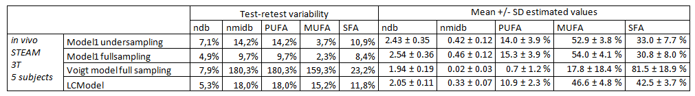
In vivo and in vitro MR spectra were quantified, according to a least-square fit implemented in a home-made MATLAB software, with the Model1 and Model2 (full sampling and undersampling) as well as with LCModel. For the oils, quantification results are compared to the theoretical known oil composition. For the AT, the variability percentage of the test-retest for each index was calculated.

Results

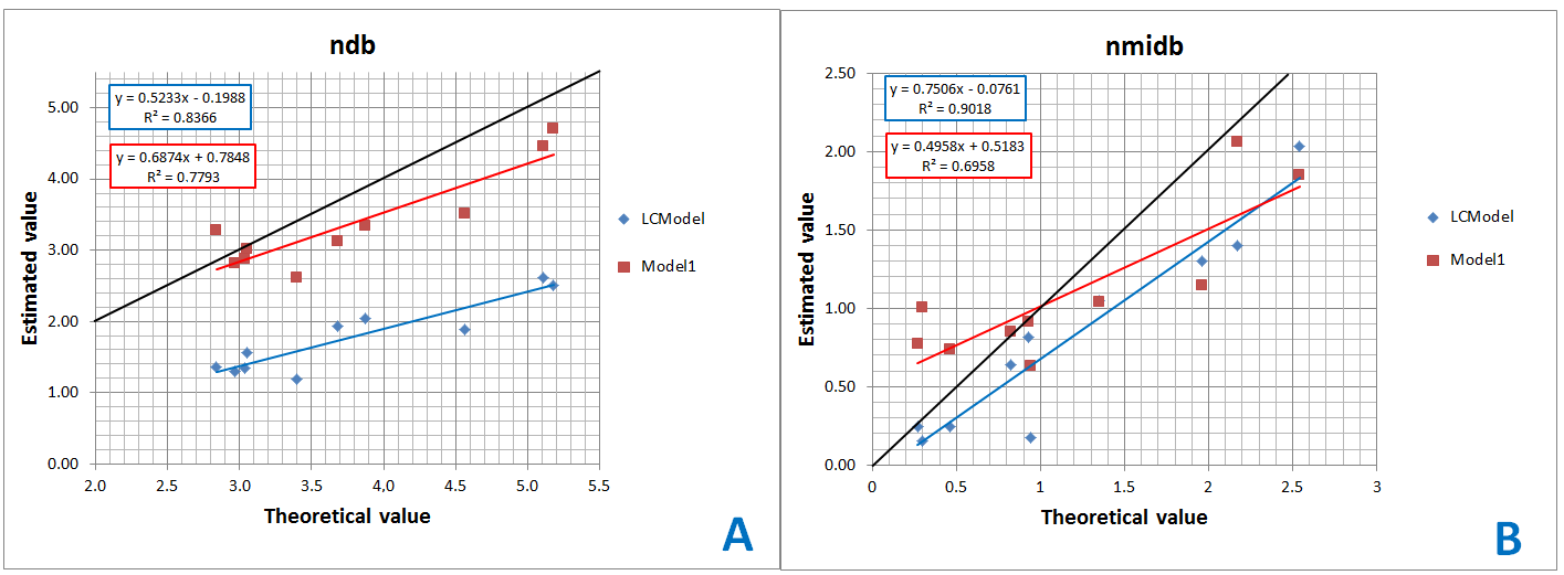
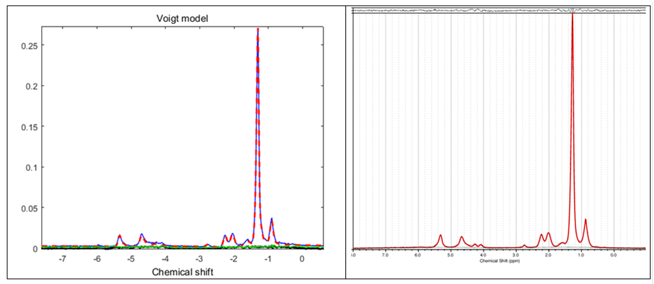
Results on the theoretical model comparison are summarized in Table2. For oil quantification results, LCModel showed the best correlation with theoretical values but under-estimated ndb. Model1 showed also good correlation and estimated values in agreement with the theoretical values when employing the undersampling (Figure1). For the in vivo results (Table3), the test-retest variability was the smallest with Model1 fullsampling. LCmodel shows good test-retest variability but with different estimated parameter values. Figure2 shows the same spectrum fitted with two different models who lead to different results despite both showing small residual.

Discussion/conclusion

This work demonstrates that, in the particular case of the lipid MRS quantification, the model function simplification (here by linking, from prior knowledge, the peak amplitude) appear to be key leverage point to increase the precision of the result. Constraints and prior knowledge as well as the time sampling selection also seem to impact the bias of the estimation and need to be further investigated.

Acknowledgements

This work was performed within the framework of the LABEX PRIMES (ANR-11-LABX-0063) of Université de Lyon, within the program "Investissements d'Avenir" (ANR-11-IDEX-0007) operated by the French National Research Agency (ANR), IHU Opera et PHRC-IR Visfatir.

References

¹Mosconi E, Sima DM, Osorio Garcia MI, Fontanella M, Fiorini S, Van Huffel S and Marzola P. Different quantification algorithms may lead to different results: a comparison using proton MRS lipid signals. NMR Biomed (2014). 27:431-443.

²Reid J G, Structural identifiability in linear time-invariant systems. IEEE Trans. Automat. Control. (1977). 22:242–246.

³Leporq B, Lambert SA, Ronot M, Vilgrain V, Van Beers BE. Quantification of the triglyceride fatty acid composition with 3.0 T MRI. NMR Biomed (2014). 27(10):1211-21.

⁴Ratiney, H., A. Bucur, M. Sdika, O. Beuf, F. Pilleul, and S. Cavassila. Effective Voigt Model Estimation Using Multiple Random Starting Values and Parameter Bounds Settings for in Vivo Hepatic 1H Magnetic Resonance Spectroscopic Data. In 5th IEEE International Symposium on Biomedical Imaging: From Nano to Macro (2008). ISBI 2008, 1529–32, 2008.

⁵Hamilton G, Yokoo T, Bydder M, Cruite I, Schroeder ME, Sirlin CB, Middleton MS. In vivo characterization of the liver fat 1H MR spectrum. NMR Biomed (2011). 24: 784–790.

⁶Garaulet M, Hernandez-Morante JJ, Lujan J, Tebar FJ, Zamora S. Relationship between fat cell size and number and fatty acid composition in adipose tissue from different fat depots in overweight/obese humans (2006).International Journal of Obesity. 30(6):899-905.

Figures

Table 1:Knowledge of the theoretical relative amplitude of the resonance associated to the chemical structure of a typical triglyceride can be either injected in the model (Model1) or be used a posteriori for fat composition assessment (Model2). frequency shift of each resonance k; ndb number of double bonds; nmidb number of methylene-interrupted double bonds; number of protons of fat spectrum component k in terms of ndb and nmidb with fixed [2,5]. Definition of PUFA, MUFA and SFA calculations with parameters estimated with the two models studied and their measurement uncertainty calculations

Table 2 : Results of measurement uncertainty calculations of ndb, nmidb PUFA, MUFA and SFA with two set of parameters: in vitro parameters used correspond to theoretical values for sesame oil, in vivo parameters correspond to the excepted fatty acid composition of human subcutaneous abdominal adipose tissue (18% PUFA 54.6% MUFA and 27.4% SFA [6]). The condition number of J explodes in the case of the Model2. In case of Model1, the undersampling enables to reduce the condition number of J for “in vitro”. Uncertainties were good for each model but increased when J is ill conditioned.

Table 3: For in vivo measurements, test-retest variability was calculated ($$$VAR=\frac{1}{N}\sum_1^N\frac{|test_i-retest_i|}{(test_i+retest_i)/2}*100$$$). According to Garaulet M et al.⁶ the fatty acid composition of human subcutaneous abdominal adipose tissue is expected to be around 18% PUFA 54.6% MUFA and 27.4% SFA. Model1 seems to have the best results with the least variability and estimated values closed to the theoretical values.

Figure1: Estimated values in function of theoretical values for ndb (A) and nmidb (B) from in vitro MRS acquired with a PRESS at 4.7T on 10 vegetal oils (peanut, avocado, canola, hazelnut, walnut, pistachio, grape-seed, sesame, sunflower and olive). Black line represents the relation y=x. Both LCModel (in blue) and Model1 undersampling (in red) show a good correlation between estimated values with theoretical values (Pearson coefficients for LCModel: $$$r_{ndb}=0.91$$$ and $$$r_{nmidb}=0.95$$$; for Model1 $$$r_{ndb}=0.88$$$ and $$$r_{nmidb}=0.83$$$). Despite the good correlation LCModel under-estimated ndb values for in vitro measurements. Model1 have estimated values in a closer agreement with the theoretical values.

Figure 2: In vivo MRS fitted with two models (Voigt model at the left and LCModel at the right). For both model, the fitted curve is in red and the residual (residual in back and absolute residual in green for the left spretrum and for the right sprectrum the residual is just on the top) is very small. For this example, fatty acid compositions found with the two models are clearly differents (3.8% PUFA, 43% MUFA and 53.6% SFA with the Voigt model and 9.6% PUFA, 50% MUFA and 40.5% SFA with LCModel).

Proc. Intl. Soc. Mag. Reson. Med. 25 (2017)

5483