5479
Ghostbusters for MRS: Automatic Detection of Ghosting Artifacts using Deep Learning1Depts. Radiology and Clinical Research, University of Bern, Bern, Switzerland
Synopsis
Ghosting artifacts in spectroscopy are problematic since they superimpose with metabolites and lead to inaccurate quantification. Detection of ghosting artifacts using traditional machine learning approaches with feature extraction/selection is difficult since ghosts appear at different frequencies. Here, we used a “Deep Learning” approach, that was trained on a huge database of simulated spectra with and without ghosting artifacts that represent the complex variations of ghost-ridden spectra. The trained model was tested on simulated and in-vivo spectra. The preliminary results are very promising, reaching almost 100% accuracy and further testing on in-vivo spectra will hopefully confirm its ghost busting capacity
Introduction:
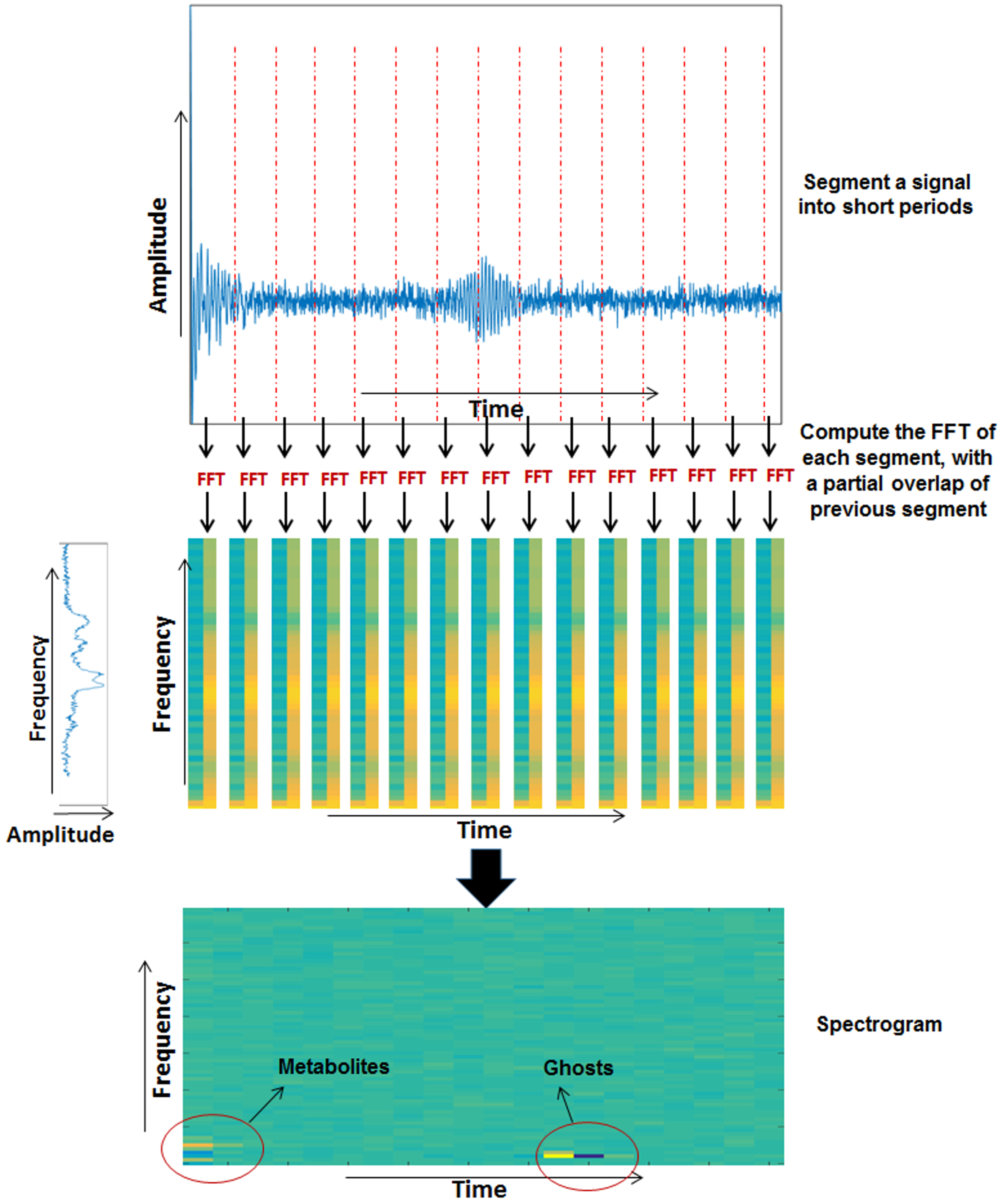
In spectroscopy, so-called ghosting artifacts appear in the spectrum due to refocusing of unwanted echoes. These ghosts are problematic because they superimpose with metabolite peaks at varying frequencies and may thus preclude reliable area estimation. Automatic ghost detection using standard machine learning methods is challenging since ghosts appear at different frequencies and are difficult to catch as specific features by standard feature extraction techniques. Deep learning techniques offer a set of algorithms that help to build deep neural network structures with multiple hidden layers and pertinent parameters extracted automatically as high level features. Hence, deep learning eases the challenge of feature engineering and helps with parameterizing neural networks. Here, we simulated spectra with and without ghosts, converted them to 2D spectrograms (Figure‑1), used them to train deep convolutional neural networks (D-CNNs), and then tested on simulated and in-vivo spectra.Methods:
Brain spectra were simulated as in Ref.(1). Ghosting artifacts with varying linewidths and amplitudes were simulated and added randomly with different time and frequency shifts.
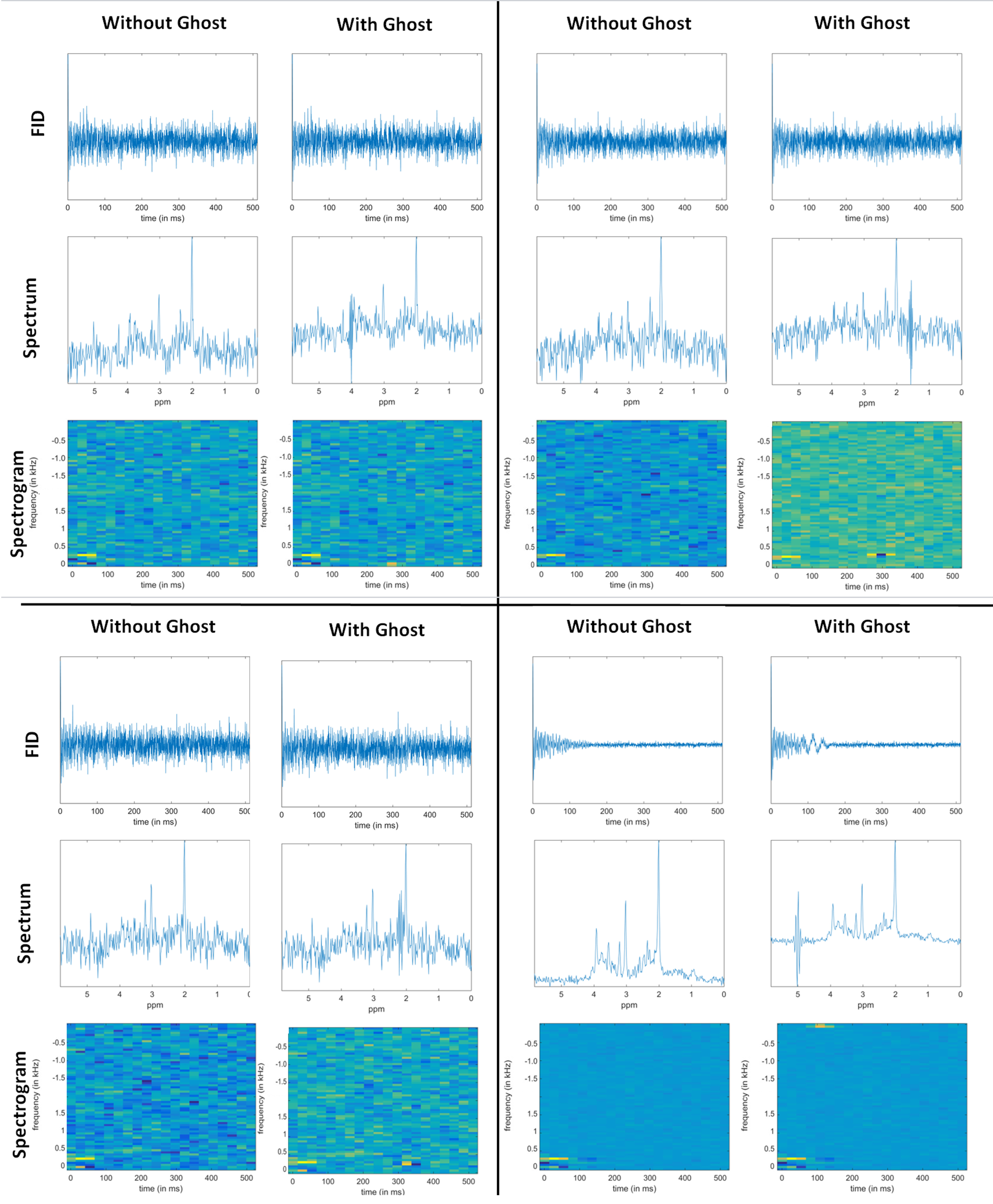
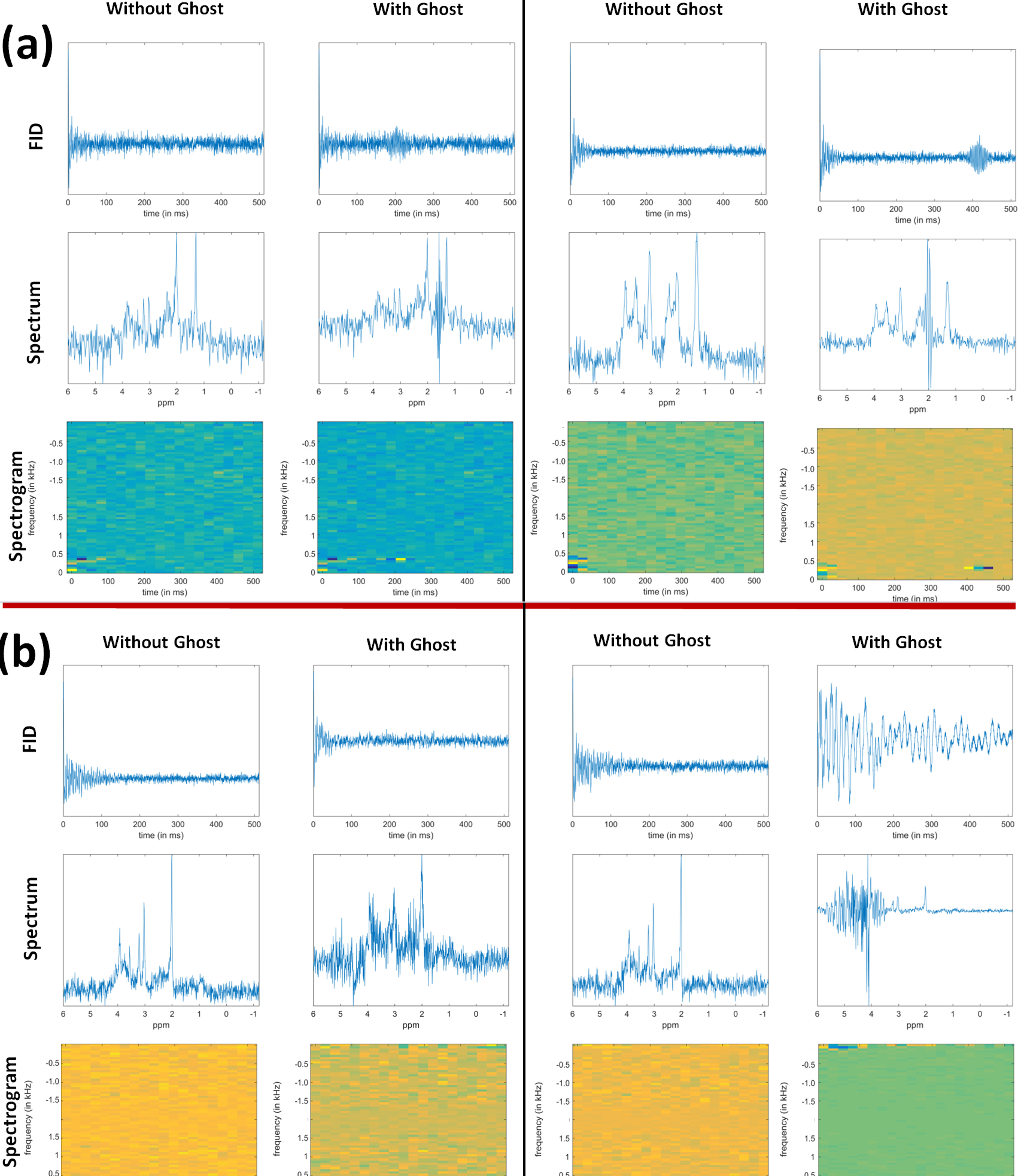
Two cohorts of spectra, labeled Group‑1 and Group‑2 (both consisting of 15000 spectra with and 15000 without ghosts) were created. Group‑1 consisted of spectra with the same brain metabolite content, but varied in linewidth (LW) and SNR (Figure‑2). Group‑2 contains spectra with variations in metabolite concentration and variable baseline (MMBL) and lipid contributions (Figure‑3a). In analogy to a Gabor transform but with inherent reduction in data-size, these were then converted into spectrograms2 (Figure‑1).
We used the Keras library3 on top of the Theano4 backend to build our deep learning network. We first started with fully connected neural network(FCN). Then, additional layers of FCN were added (up to 6 layers) and trained on simulated spectra. Upon finding rather poor performances, we started building a model using the most popular kind of deep learning models, called D-CNNs, which have succeeded in image recognition competitions5,6. We tried different layer (n=2,3,4) and filter sizes for each layer, containing two or three convolutional filters on top of FCN. The optimized architecture (batch size=50, epochs=5) for our study were trained on the Amazon Web Service infrastructure7 to speed up training, using complex spectrograms as input (Figure‑4).
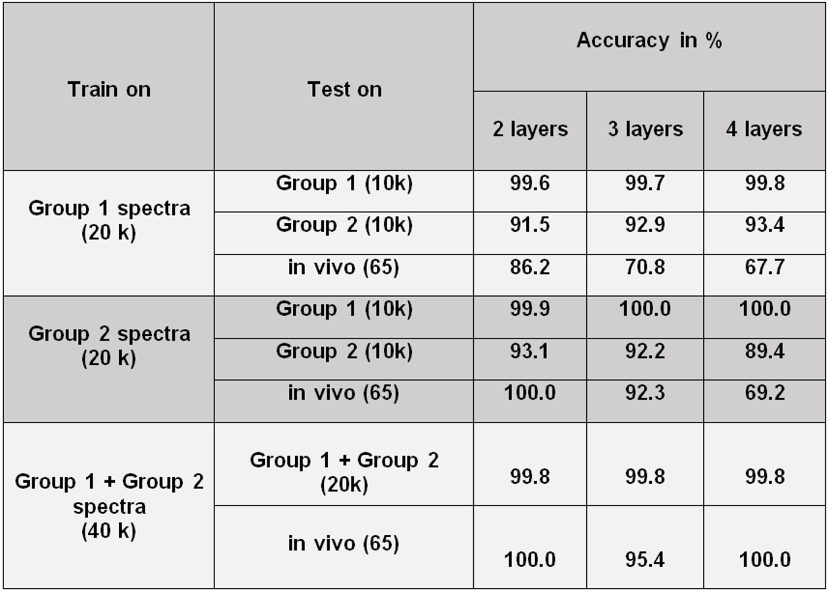
The trained D-CNNs were tested on Group‑1 (10k spectra), Group‑2 (10k), combined Group‑1+Group‑2 (20k) and in-vivo (65) data. The in-vivo spectra were preprocessed in jMRUI to remove the water residues8. 32% of the in-vivo data had ghosting artifacts (Figure‑3b).
Results:
All results are summarized in Table 1. The accuracy of D-CNNs trained with Group‑1 spectra when tested on similar spectra was extremely good; however for Group‑2 spectra the accuracy dropped to ~92%, and was poor for in-vivo spectra.
The D-CNNs trained on Group‑2 performed well when tested in-vivo, with the accuracy reaching 100% for 2 layers, however for Group‑1, they did not do well.
In order to cover as much as possible of the variance expected for pathologic in-vivo spectra, new D-CNNs were trained combining Group‑1 and Group‑2 spectra, which surprisingly yielded ~100 % accuracy both for simulated and in-vivo spectra.
Discussion:
In D-CNNs each network layer9 acts as a detection filter (feature extraction) for the presence of specific features in the spectra. The first layers detect large features, like metabolite components etc. The subsequent layers find increasingly smaller more abstract features like the position of ghosts or noise. The final layers then match input spectra with all the specific features detected by previous layers and the final prediction is a weighted sum of all of them. Thus, D-CNNs are able to model complex variations and behavior, which is now reflected in the good performance for artifact detection.
For the detection of ghosts, we converted spectra to spectrograms that provide an image-like 2D time-frequency representation of spectra that seems well-suited for definition of ill-timed spectral contributions. D-CNNs are known to be well-suited for images with RGB channels as input; here we used the real and imaginary parts of spectrograms as a two-channel input to D-CNNs yielding excellent artifact recognition performance in the tested cases. This initial trial will be extended to larger sets of in-vivo spectra (including residual water, other acquisition parameters) and the detection of other artifacts. General use of deep learning techniques for in-vivo spectroscopy is limited to applications where thousands of spectra can be provided for training and testing, thus to cases where simulations can fully cover in-vivo feature space.
Conclusion:
In this study, we show that it is possible to use deep learning to detect ghosting artifacts for in-vivo MRS. Initial results show promising performance and motivate further extensions of the methods and applications.
Acknowledgements
This research was carried out in the framework of the European Marie-Curie Initial Training Network, ‘TRANSACT’, PITN-GA-2012-316679, 2013-2017 and also supported by the Swiss National Science FoundationReferences
1. Kyathanahally SP, Kreis R. Forecasting the quality of water-suppressed 1H MR spectra based on a single-shot water scan. Magn. Reson. Med. 2016 Sep 8. doi: 10.1002/mrm.26389.
2. Simpson AJR. Deep Transform: Cocktail Party Source Separation via Complex Convolution in a Deep Neural Network. 2015, arXiv:1504.02945v1 [cs.SD].
3. Chollet F. Keras. https://github.com/fchollet, Last accessed : Nov 2016.
4. Al-Rfou R, Alain G, Almahairi A, et al. Theano: A Python framework for fast computation of mathematical expressions. arXiv e-prints 2016;abs/1605.0:19.
5. Russakovsky O, Deng J, Su H, et al. ImageNet Large Scale Visual Recognition Challenge. Int. J. Comput. Vis. 2015;115:211–252.
6. Simonyan K, Zisserman A. Very Deep Convolutional Networks for Large-Scale Image Recognition. Int. Conf. Learn. Represent. 2015:1–14.
7. Amazon Inc. Amazon Web Service. http://aws.amazon.com/, Last accessed : Nov 2016
8. Naressi A, Couturier C, Castang I, Beer R De, Graveron-Demilly D. Java-based graphical user interface for MRUI , a software package for quantitation of in vivo/medical magnetic resonance spectroscopy signals. Comput Biol Med. 2001;31:269–286.
9. Yosinski J, Clune J, Nguyen A, Fuchs T, Lipson H. Understanding Neural Networks Through Deep Visualization. Int. Conf. Mach. Learn. - Deep Learn. Work. 2015 2015:12.
10. Döring A, Adalid Lopez V, Brandejsky V, Boesch C, Kreis R, Diffusion weighted MR spectroscopy without water suppression allows to use water as inherent reference signal to correct for motion-related signal drop. In: Proc. Intl. Soc. Mag. Reson. Med. 24 (2016) #2395
Figures