5478
Quality Control of MRSI data using efficient data labelling1SCAN / Neuroradiology, University Hospital Bern (Inselspital), Bern, Switzerland
Synopsis
MRSI-data frequently contains bad-quality spectra, what can prevent proper quantification and consequently lead to data misinterpretation. Machine-learning based methods have been proposed for automatic quality control of MRSI-data with performance levels identical to expert’s-manual-checking and that can classify thousands of spectra in a matter of a few seconds. Besides this, a considerable amount of time needs to be spent labelling data required to train these algorithms. Here we present a method that allows to actively select those spectra that carry the most information for the classification, allowing to reduce drastically the amount of time needed for labelling.
Introduction
Machine-learning based methods for quality-control of MRSI-data1–4 have shown performance-levels identical to expert’s manual-checking and are fast, automatic and produce systematic results. Besides its time-saving potential, to train these classifiers considerable amounts of time need to be spent labelling training-data.
Active-learning5,6 is capable of increasing labelling-efficiency by allowing the learning-method to actively select the examples with more information for labelling. The selection-strategy tested here was uncertainty-sampling7, a method that gives priority to those examples whose class membership is more uncertain.
In this work, we report the results of an experiment where the use of active-learning with uncertainty-sampling was tested in automatic-quality-control of MRSI-data. Data that had been completely labelled was used to run several simulations where the spectra were gradually selected and added to the training-set. In these simulations, the selection of cases from a completely labelled dataset simulates the partial-labelling of the data.
Methods
MRSI-data was acquired at 1.5T (Siemens Aera, Avanto) using PRESS, CHESS, TE/TR=135/1500ms, 32x32 resolution (original 12x12). 58 MRSI-recordings from 18 brain-tumour patients acquired pre- and post-operatively, were included in the study. The measurements were performed conforming to local and national ethical regulations. Only the 14216 spectra from within the PRESS-box were used. Residual-water-peak-removal was performed prior to feature extraction (jMRUI’s HLSVD). All spectra were manually labelled in either “Accept” or “Reject”. The features for rejecting spectra were: “ghosting” artifacts, bad-shimming, low-SNR, lipid-contaminations, strongly deviating phase, and post-operative-derived artifacts. The complete-labelling was performed in two steps. First, the experts labelled the spectra independently. Then, they revised together those spectra in which there was disagreement, reaching a consensus-labelling. The resulting consensus-labels constituted the ground-truth used for training and testing the automatic-classifiers. A total of 47 features were extracted from the magnitude time-domain (TD) and frequency-domain (FD) signals2. A random-forest8,9 (RF) classifier (“R” implementation, 200 trees, maximum depth) was used for the automatic assessment.
The simulations that were used to test the active-learning with uncertainty-sampling approach were performed in following way:
For every patient i (out of 18):
1. Use patient i as validation-set and add remaining patients to a set-A;
2. Shuffle patients’ order in set-A;
3. Add all examples from the first patient of set-A (patient 0) to the training-set;
4. Train classifier and measure performance on validation-set;
5. Until all patients from set-A have been analysed:
5.a. Classify next patient’s spectra;
5.b. Uncertainty-sampling - add all spectra to the training-set that satisfy: $$0.5-α ≤ p(y=”Accept”|x) < 0.5+α$$, where $$$p(y=”Accept”|x)$$$ is the probability outputted by the classifier of an example being considered as having acceptable quality by a rater, given its features.
5.c. Retrain classifier and evaluate performance on validation-set.
Given that the order of the patients in set-A has an influence on the evolution of the performance of the classifier as the training sample size increases, the order of the patients was shuffled (step 2) and the simulation was repeated 50 times. Five different $$$α$$$-values were tested: 0.1, 0.2, 0.3, 0.4 and 0.5, representing 0.5 the case where all data is labelled and added to the training-set. For each $$$α$$$ and number of patients added to the training set (steps 3 and 5.b), the mean cross-validated accuracy, sensitivity and specificity across the 50 repetitions were determined.
Results/Discussion
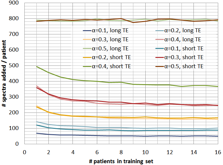
Figure 1 shows the mean
number-of-spectra added to the training-set for every new patient, for
different $$$α$$$-values and for short and long-TE, showing how $$$α$$$
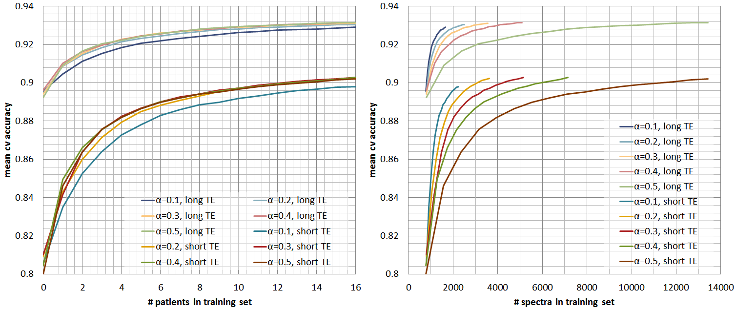
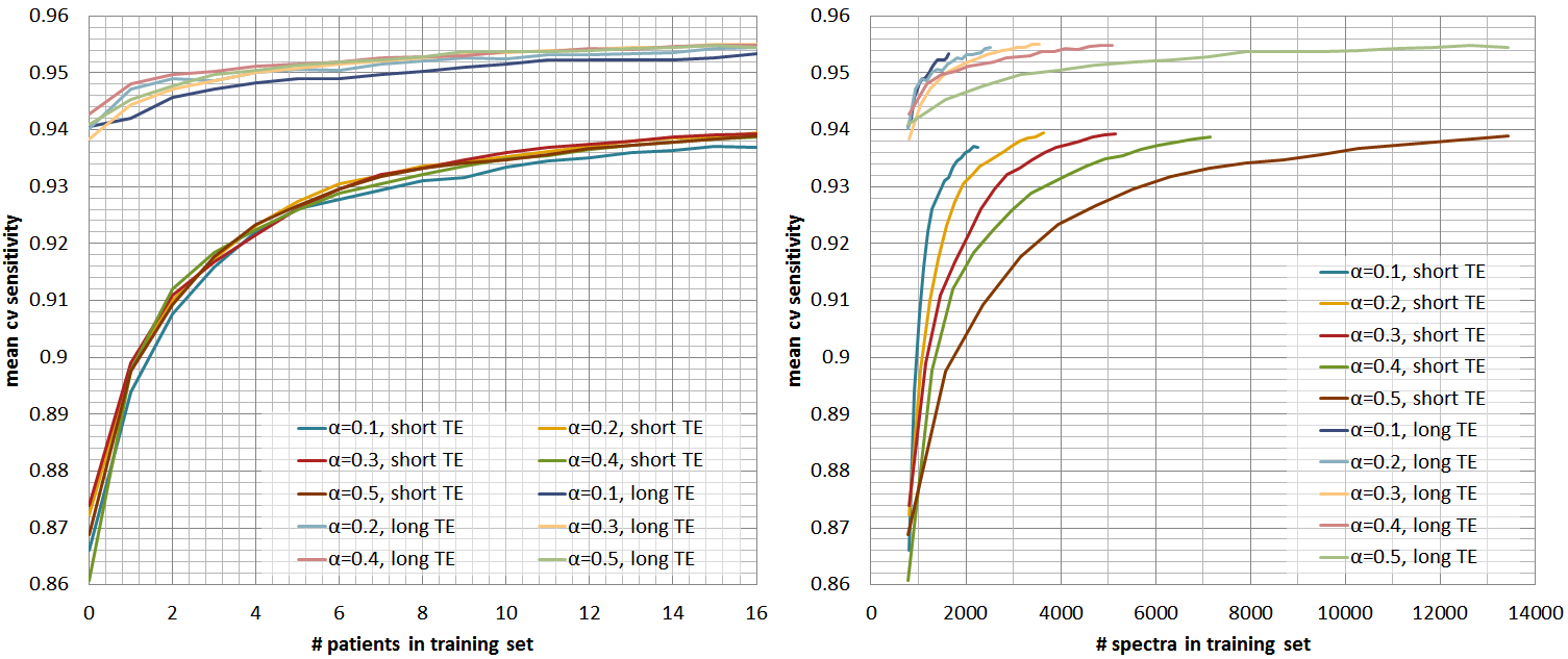
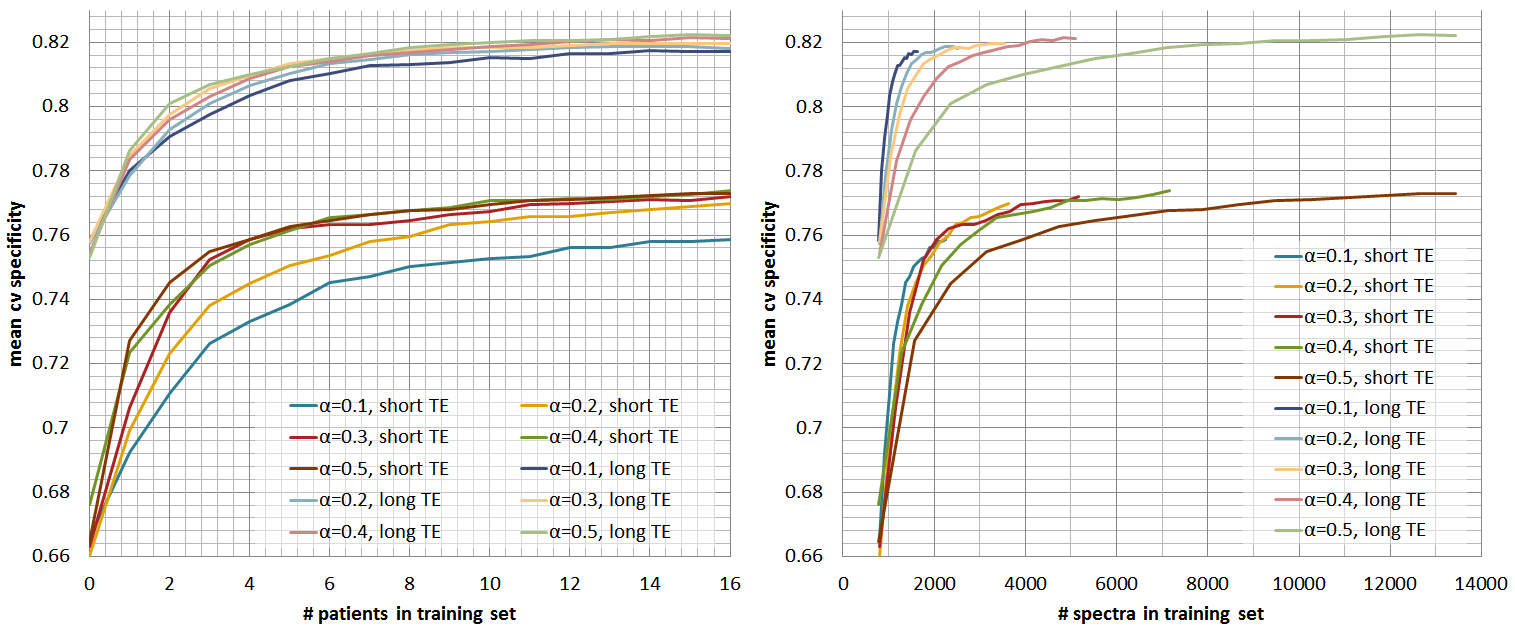
controls the amount of data that is labelled per grid. Figures 2, 3, and 4 show
respectively the mean cross-validate accuracy, sensitivity and specificity for
different $$$α$$$-values and for short and long-TE, in function of the
number-of-patients added to the training-set(left) and the number-of-spectra
added to the training-set(right). Here we see that the proposed method allows considerable
reductions in labelled data with no or little impact in performance, still
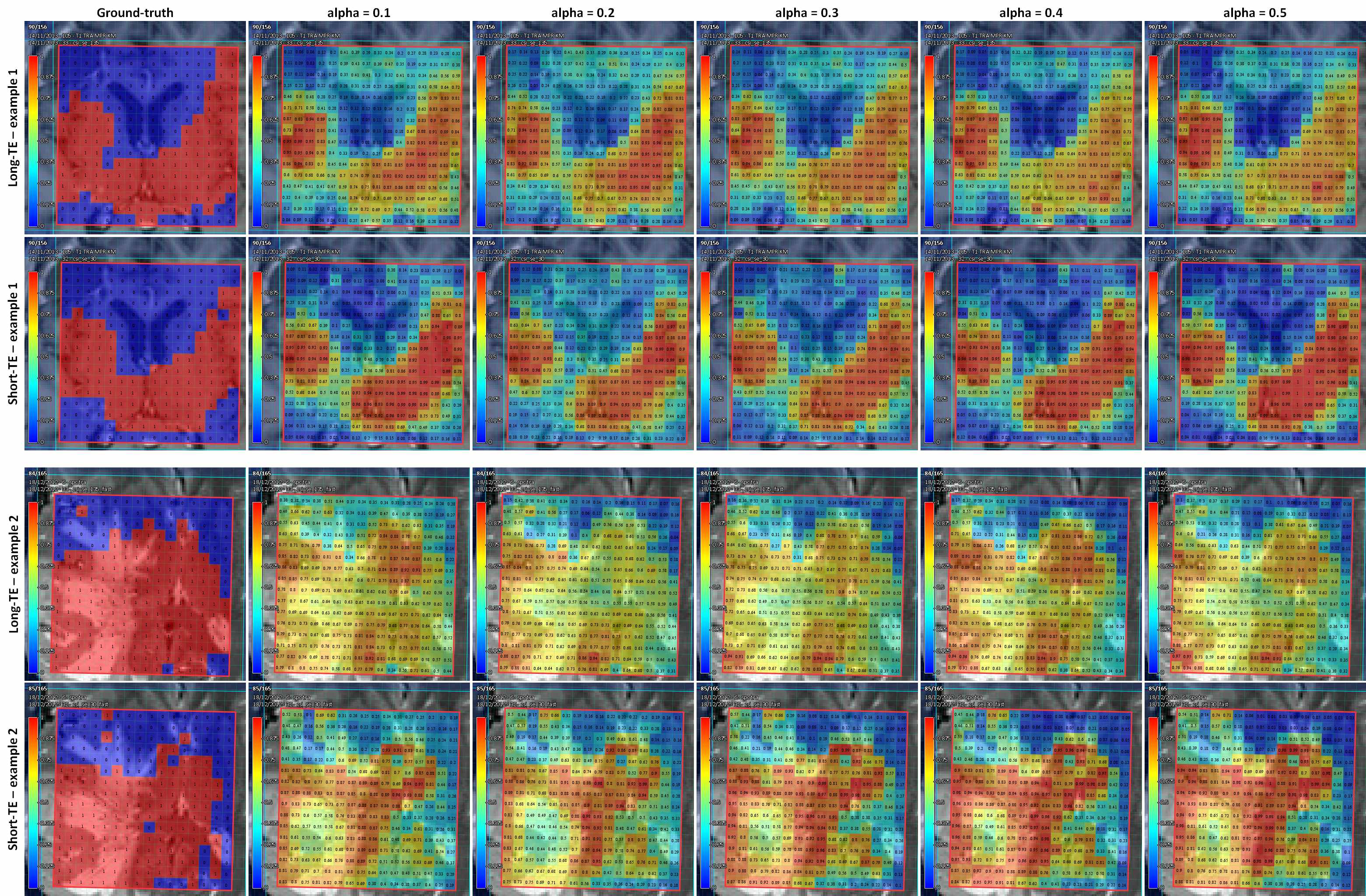
specificity is more affected than sensitivity. Figure 5 shows quality-maps for
both TEs of two different cases where the classifiers were trained using
different $$$α$$$-values. Here we see that despite the differences in training-set
size, the results for different $$$α$$$ are quite similar.
Conclusion
The proposed method allows to drastically improve the labelling efficiency in MRSI-quality-control. This method might be especially relevant for high resolution MRSI (e.g. EPSI, SPICE), in which huge number of spectra are generated in each acquisition and where not only manual assessment is impossible but labelling completely a few or even one MRSI dataset might be simply not feasible. In those cases, besides automatic classifiers for quality control being needed, the optimization of the labelling procedure becomes a must.Acknowledgements
This work was funded by the EU Marie Curie FP7-PEOPLE-2012-ITN project TRANSACT (PITN-GA-2012-316679) and the Swiss National Science Foundation (project number 140958).References
1. Pedrosa de Barros N, McKinley R, Knecht U, Wiest R, Slotboom J. Automatic quality assessment of short and long-TE brain tumour MRSI data using novel Spectral Features. Proc Intl Soc Mag Reson Med 24. 2016.
2. Pedrosa de Barros N, Mckinley R, Knecht U, Wiest R, Slotboom J. Automatic quality control in clinical 1 H MRSI of brain cancer. NMR Biomed. 2016;(August 2015). doi:10.1002/nbm.3470.
3. Wright AJ, Kobus T, Selnaes KM, et al. Quality control of prostate 1 H MRSI data. NMR Biomed. 2013;26(2):193-203. doi:10.1002/nbm.2835.
4. Menze BH, Kelm BM, Weber MA, Bachert P, Hamprecht FA. Mimicking the human expert: Pattern recognition for an automated assessment of data quality in MR spectroscopic images. Magn Reson Med. 2008;59(6):1457-1466. doi:10.1002/mrm.21519.
5. Maiora J, Ayerdi B, Graña M. Random forest active learning for AAA thrombus segmentation in computed tomography angiography images. Neurocomputing. 2014;126:71-77. doi:10.1016/j.neucom.2013.01.051.
6. Tuia D, Ratle F, Pacifici F, Kanevski MF, Emery WJ. Active learning methods for remote sensing image classification. IEEE Trans Geosci Remote Sens. 2009;47(7):2218-2232. doi:10.1109/TGRS.2008.2010404.
7. Lewis DD, Gale W a. A Sequential Algorithm For Training Text Classifiers. Proc 17th Int Conf Res Dev Inf Retr. 1994:3-12. doi:10.1145/219587.219592.
8. Liaw a, Wiener M. Classification and Regression by randomForest. R news. 2002;2(December):18-22. doi:10.1177/154405910408300516.
9. Breiman L. Random forests. Mach Learn. 2001;45(1):5-32. doi:10.1023/A:1010933404324.
Figures