5458
The ultimate local SAR in realistic body models: Preliminary convergence results1Radiology, Massachusetts General Hospital, Charlestown, MA, United States, 2Harvard Medical School, Boston, MA, United States, 3Cadence Design Systems, Feldkirchen, Germany, 4Skolkovo Institute of Science and Technology, Moscow, Russian Federation, 5Harvard-MIT Division of Health Sciences Technology, Cambridge, MA, United States, 6Institute for Medical Engineering and Science, Massachusetts Institute of Technology, Cambridge, MA, United States, 7Dept of Electrical Engineering and Computer Science, Massachusetts Institute of Technology, Cambridge, MA, United States
Synopsis
We extend our previously reported methodology for computation of the ultimate signal-to-noise ratio in realistic body models to the computation of the ultimate specific absorption rate (SAR) in the head of the Duke body model at 3 Tesla. We optimize 90° magnitude least-squares RF pulses subject to hundreds of thousands of SAR constraint for increasing numbers of electromagnetic fields in the basis set. As the size of the basis set increases, we show that the local SAR decreases toward a value that we call the “ultimate local SAR”.
Target audience
RF engineers and MRI physicists.Purpose
Recently, we have proposed a methodology for the computation of the ultimate signal-to-noise in MRI in realistic body models [1]. We extend this approach to the computation of the ultimate local specific absorption rate (SAR) in the head of the Duke body model [2] at 3 Tesla.Methods
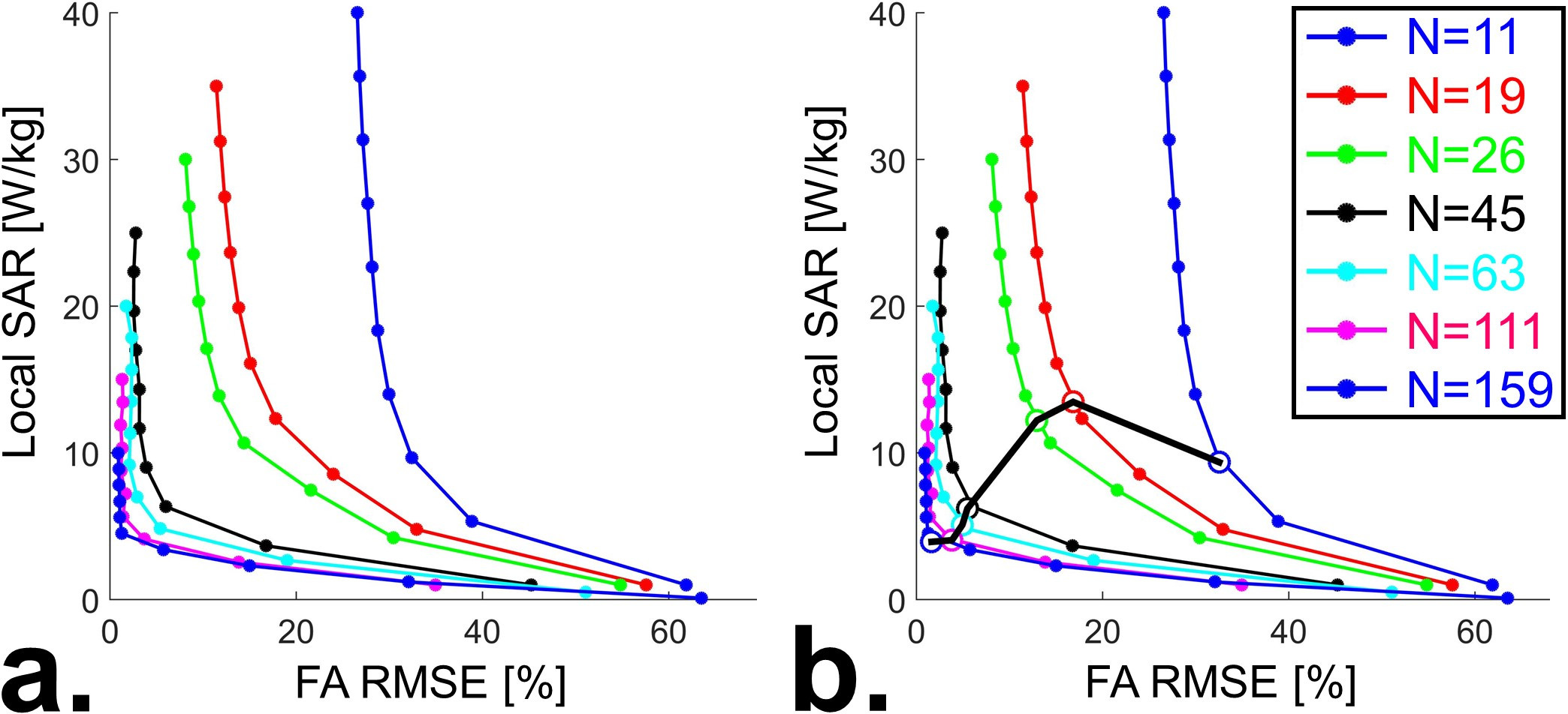
Basis fields generation: For generation of a complete basis set of the solution to Maxwells’s equations in the head of the Duke body model (Fig. 1a), we use the same technique that we used previously [1]. STEP #1: We place a large number of electric and magnetic dipoles at a minimum distance of 3 cm (Fig. 1c) to the head and we excite those dipoles using random amplitudes and phases. No dipoles are placed below the neck since no coils can be placed there. STEP #2: We compute the incident fields created by the random dipole excitations. STEP #3: We compute the scattered component of the electric field in Duke’s head using the fast MARIE electromagnetic solver [3]. STEP #4: We sum the incident and scattered electric field components to obtain the total fields. Pulse design: We optimize slice-selective RF-shimming 90º degree, 20% duty-cycle pulses using a magnitude least-square objective [4] that accounts for the full Bloch equation dynamics (i.e., we do not use the small tip-angle approximation) [5]. We incorporate SAR constraints for every voxel in the body model, which results in 193,542 constraints (i.e. we do not compress the SAR matrices using the VOP algorithm). We provide analytical expressions of the Jacobian of the objective (Bloch) and constraint functions (SAR) for faster convergence. To minimize computation time, we parallelize these computations using a Tesla K20 GPU. Ultimate local SAR analysis: For a given basis-set (i.e., fixed N), we optimize a series of pulses corresponding to varying local SAR constraints (L-curve). We then fit the L-curve to an exponential model (sum of two exponentials) and use the fit to determine the “optimal point” of the curve as the point with the greatest curvature. Finally, we report the flip-angle error and local SAR of optimal points associated with increasing N. Temperature simulation: We compute the steady-state temperature of the optimal SAR maps using a Crank-Nicholson discretization of the Pennes bio-heat equation [6].Results
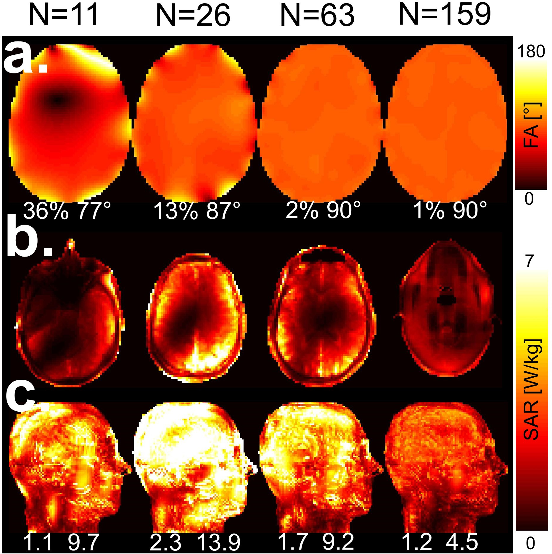
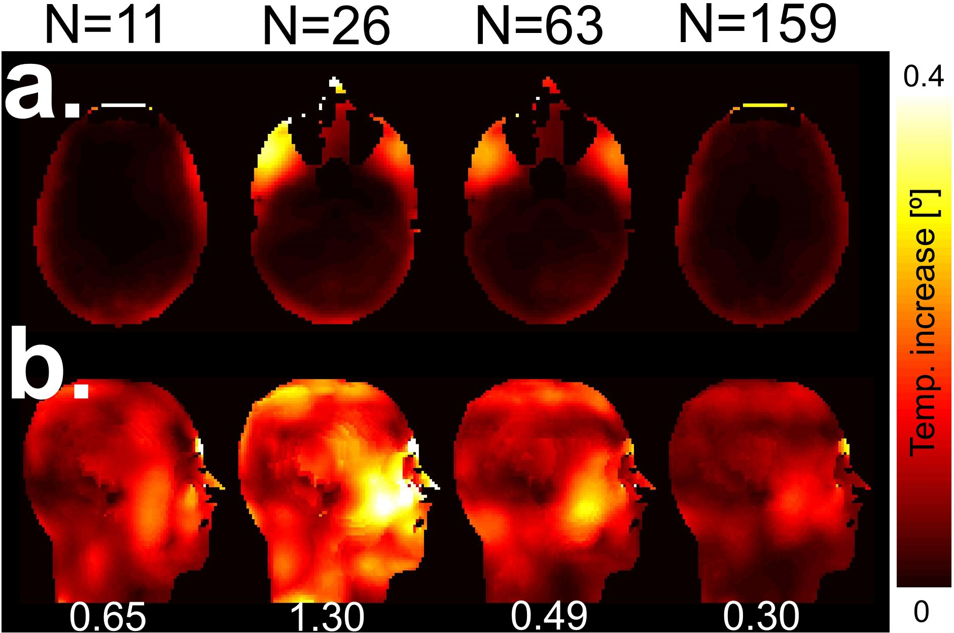
Fig. 2 shows that, as expected, L-curves associated with increasing large basis sets (i.e., increasing N) are closer and closer to the origin of the RMSE vs local SAR graph. The L-curves of Fig. 2 for increasing N display the “typical L-shape” with a clear optimal point. Fig. 3 shows the local SAR and flip-angle error of these optimal points for increasing N. The RMSE converges toward zero, which is another way to say that the flip-angle maps approach the optimal, perfectly flat 90º flip-angle distribution (Fig. 4a). However, the local SAR graph seems to plateau toward a value which we call the “ultimate local SAR”, which is this work is equal to ~5 W/kg. However, it is clear that the basis sets used in this work are not “large enough” to approximate the value of the ultimate local SAR with a high degree of accuracy and confidence. Visual comparison of the maps in Figs. 4 and 5 shows that the SAR and temperature distributions are very different, which is due to the non-uniform perfusion map in this body model (see Fig. 1b. This result is in agreement with previous studies [7]). This indicates that the ultimate SAR is likely different from the ultimate temperature. We also point out that the maximum steady-state temperature of the relatively high-power pulse studied in this work is only 0.4º for N=159, which is well below the tolerated limit of 1º.Conclusion
We have proposed an approach for computation of the ultimate local SAR in realistic body models. Our results are preliminary because our SAR maps have clearly not converged to the actual ultimate SAR value. Accurate estimation of the ultimate local SAR in Duke’s head will require using larger basis sets (i.e., greater N). This is challenging however, because the high memory requirements of such large datasets are beyond the capability of our GPU card. More investigation of the differences between the ultimate SAR and the temperature distributions is also needed.Acknowledgements
R01EB006847, P41EB015896, K99EB019482References
[1] Guerin B et al. (2014). The ultimate SNR and SAR in realistic body models. Proceedings of the ISMRM, 22:617.
[2] Christ A et al. (2010). "The Virtual Family—development of surface-based anatomical models of two adults and two children for dosimetric simulations." Physics in medicine and biology 55(2): N23.
[3] Polimeridis A et al. (2014). "Stable FFT-JVIE solvers for fast analysis of highly inhomogeneous dielectric objects." Journal of Computational Physics 269: 280-296.
[4] Setsompop K et al. (2008). "Magnitude least squares optimization for parallel radio frequency excitation design demonstrated at 7 Tesla with eight channels." Magnetic Resonance in Medicine 59(4): 908-915.
[5] Massire A et al. (2013). "Design of non-selective refocusing pulses with phase-free rotation axis by gradient ascent pulse engineering algorithm in parallel transmission at 7T." Journal of Magnetic Resonance 230: 76-83.
[6] Zhao JJ et al. (2005). "A two level finite difference scheme for one dimensional Pennes’ bioheat equation." Applied Mathematics and Computation 171(1): 320-331.
[7] Boulant, N., et al. (2016). "Direct control of the temperature rise in parallel transmission by means of temperature virtual observation points: Simulations at 10.5 tesla." Magnetic Resonance in Medicine 75(1): 249-256.
Figures