Synopsis

The purpose of our study was to evaluate the spatial distribution of a gradient-pulse-to-acoustic-noise transfer function (GPAN-TF) with and without a phantom inside the bore. This study showed that the spatial distribution of GPAN-TFs with a phantom in the bore was significantly larger than that with an empty imager. The GPAN-TF spectrum for high frequency range were increased by the phantom. Therefore, the patient would be exposed to a more unpleasant sound than conventional evaluation in an empty scanner. The multipoint analysis using GPAN-TFs revealed structural differences in respective gradient coils under a situation similar to actual MR examination.

INTRODUCTION

METHODS

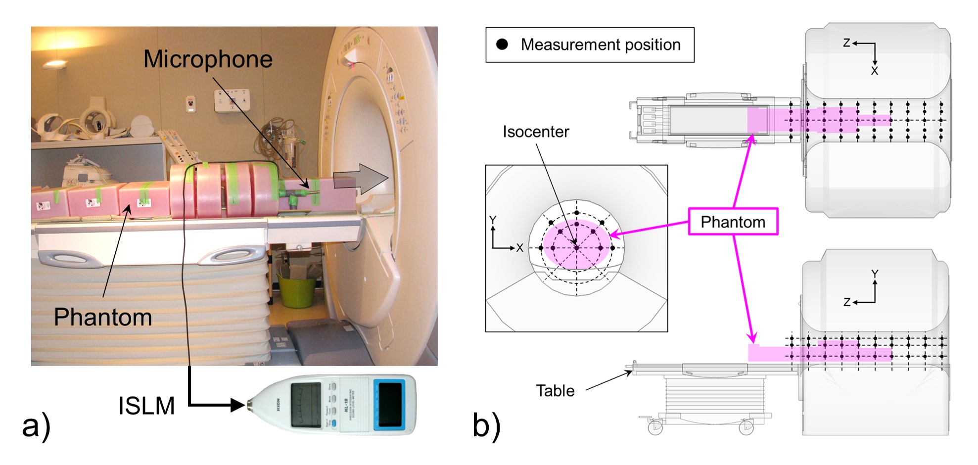
We measured sound pressure levels (SPL) in the frequency domain of a 3.0-T super-conducting MRI system (Signa Excite HDxt, General Electric Healthcare, Wisconsin, USA) when applying a simple narrower trapezoidal gradient pulse to the X, Y, and Z gradient coil. Within the manufacturer’s pulse sequence design limitations, the minimum rise and fall times and gradient pulse on-time were allowed and the maximum amplitude was allowed. Measurements were performed using a precision integrating sound level meter (NL-18, RION Co., Ltd., Tokyo, Japan) connected to an electret condenser microphone. Acoustic noise waveforms induced by a single gradient pulse were digitalized and sampled at 96 kHz; subsequent data were acquired in the frequency domain using a computational tool, including Fourier transforms. To measure peak SPL, the microphone was directed parallel to the patient axis and in a horizontal plane on the patient table (Fig. 1a). We calculated GPAN-TF [μPa/(mT/m)] in each gradient coil, i.e., X, Y, and Z-axis, by the deconvolution process.

We then compared the effect of the presence and absence of the phantom as follows: longitudinal variation in the magnet isocenter for the phantom at 10 cm intervals; spatial dependence inside the bore at 80 and 110 measurement points with and without the phantom (Fig. 1b); influence of the X, Y, and Z gradient coils; and the frequency response properties.

RESULTS

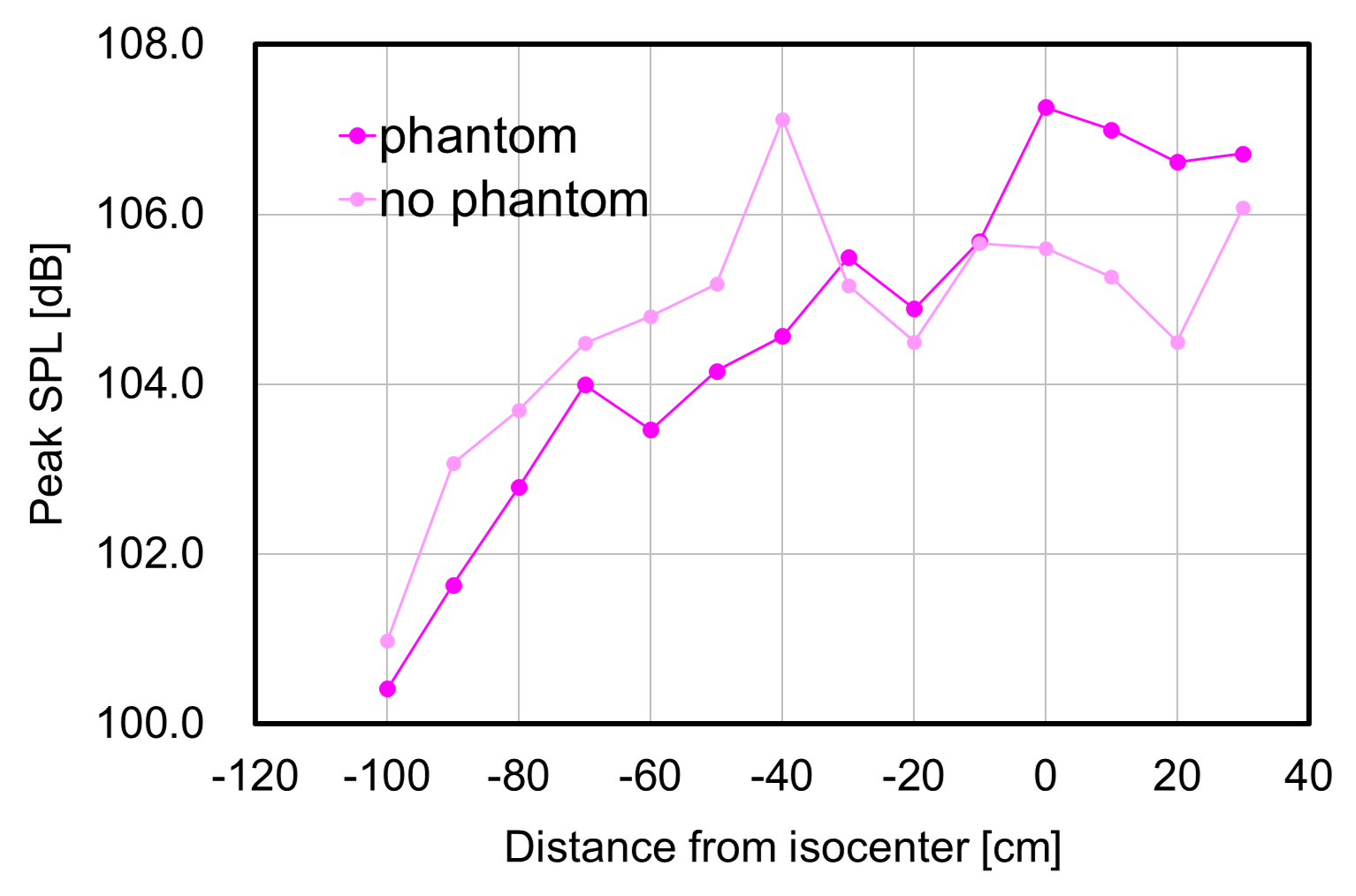
Imaging isocenter from the head to the chest region had an increased SPL of up to 5.7 dB with the phantom (Fig. 2). When the isocenter was measured from the abdomen to foot region, SPL at the left and right ear position decreased up to 6.1 dB.

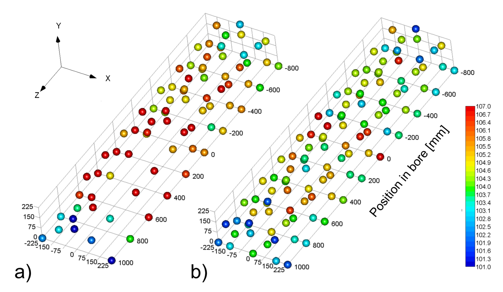
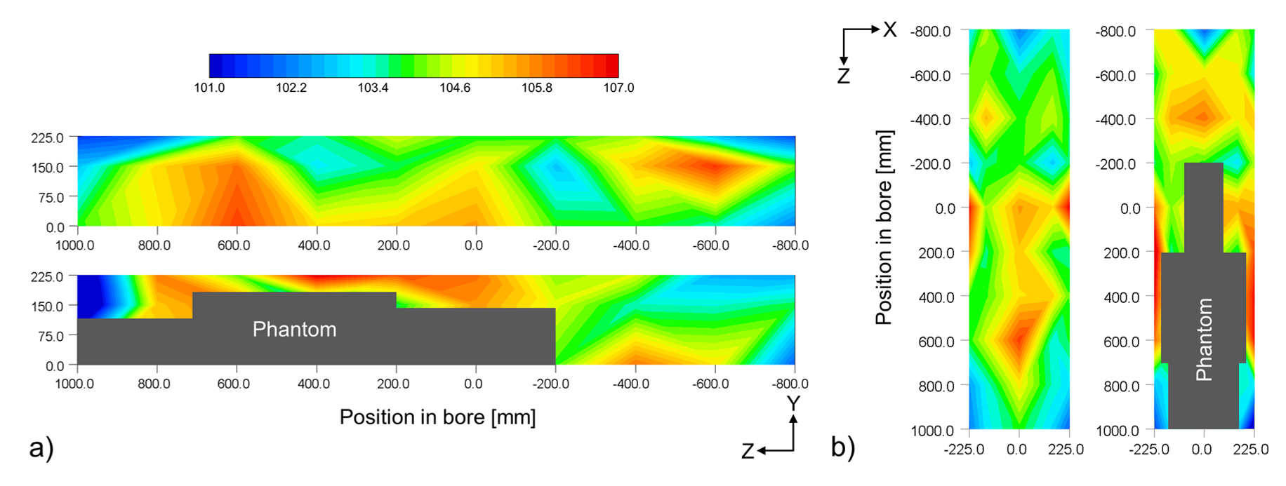
The spatial distribution of GPAN-TFs with a phantom in the bore was significantly larger than that with an empty imager, as shown in Fig. 3 (P < 0.01, paired t-test). In particular, GPAN-TFs showed a notable change when measured near the phantom (Fig. 4), and GPAN-TFs of X, Y, and Z gradient coils peaked in different positions without the phantom. The highest points of GPAN-TFs associated with the phantom also varied according to the gradient coils.

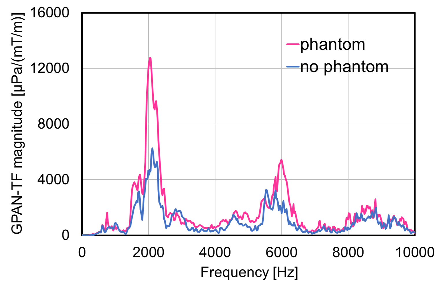
The frequency analysis of GPAN-TF indicated two peak values at approximately 2 and 6 kHz, and the peak values increased with the presence of the phantom (Fig. 5).

DISCUSSION

The presence of the phantom increased SPLs near the ear positions. When imaging the upper body, the measurement values were larger for SPLs with the phantom than those without the phantom; however, the impact decreased when imaging the lower body. This may be due to the shielding effect of the phantom itself. Moreover, the traditional measurement method of acoustic noise in MRI has the potential of underestimating the actual values.³

The GPAN-TFs of X, Y, and Z gradient coils had characteristic spatial distribution. This result shows that the “hotspot” area of GPAN-TFs may be associated with acoustic noise sources. Therefore, increasing GPAN-TF points with the phantom differed among the gradient coils. The measurement position near the phantom had a larger GPAN-TF because SPLs increased by the phenomenon of pressure doubling.⁴

The GPAN-TF spectrum two peaks for high frequency range were increased by the phantom. This result shows the patient would be exposed to a more unpleasant sound than conventional evaluation in an empty scanner. In addition, because GPAN-TFs may be influenced by local RF transmit coils and patient’s body size, detailed information requires further investigation.

CONCLUSION

Acknowledgements

References

1. Hamaguchi T, Miyati T, Ohno N, et al. Acoustic noise transfer function in clinical MRI: a multicenter analysis. Acad Radiol. 2011;18(1):101-106.

2. Price D, De Wilde J, Papadaki A, et al. Investigation of acoustic noise on 15 MRI scanners from 0.2 T to 3 T. J Magn Reson Imaging. 2001;13:288-293.

3. National Electrical Manufacturers Association. Acoustic noise measurement procedure for diagnostic magnetic resonance imaging devices. NEMA Standards Publication MS-4 2010.

4. Hedeen R, Edelstein W. Characterization and prediction of gradient acoustic noise in MR imagers. Magn Reson Med. 1997;37:7-10.