5450
Analytical Solution for Electric Field Induced Inside Ellipsoidal Conductor by Time-Varying Magnetic Fields in MRI1University of California, San Francisco, San Francisco, CA, United States
Synopsis
An analytical, closed-form solution for the electric field induced inside an ellipsoidal conductor by time-varying gradients in MRI was developed. We applied the method to calculate the electric field for an ellipsoid centered on the isocenter having the semi-axis lengths 20 cm, 15 cm, and 40 cm in LR, AP, and SI directions. We observed that, due to the geometry, ramping up on the Y-axis resulted in the highest electric field intensity. Furthermore, we found that, when the ellipsoid is shifted in the SI direction, the electric field intensity increases approximately 100%.
Introduction
An analytical, closed-form solution for the electric field induced inside an ellipsoid conductor by time-varying gradients was developed by solving Maxwell's equations under quasistatic assumptions. The approach would enable us to estimate the induced electric field in real-time for any given gradient waveforms without performing numerical simulations.
Methods
The Maxwell-Faraday equation in differential form is written as $$\nabla \times \mathbf{E}\left(x,y,z,t\right) = - \frac{\partial{\mathbf{B}\left(x,y,z,t\right)}}{\partial{t}}$$ which states that an applied time-varying magnetic field $$$\mathbf{B}$$$ will induce a spatially-varying electric field $$$\mathbf{E}$$$. We can write both the vector fields in terms of potentials:$$ \label{vmp}\mathbf{B} = \nabla \times \mathbf{A}$$ and $$\label{sep}\mathbf{E} = -\nabla V - \frac{\partial\mathbf{A}}{\partial t},$$ where $$$\mathbf{A}$$$ is the vector magnetic potential and $$$V$$$ is the scalar electric potential. Under quasistatic assumptions, we can find the electric field $$$\mathbf{E}$$$ by solving a Neumann boundary value problem: $$\mathbf{E} \cdot \mathbf{n} \mid_{\partial \Omega} = 0, \quad \nabla V = 0,$$ where $$$\partial \Omega$$$ represents the ellipsoid and $$$\mathbf{n}$$$ is the outward unit normal vector on the ellipsoid surface (Fig. 1). We used the concomitant magnetic field model developed by Bernstein el al. [1] to represent the time derivative of the magnetic field $$$\mathbf{B}$$$ as a polynomial function of the spatial coordinates and applied linear gradients: $$\frac{\partial \mathbf{B}}{\partial t} = \begin{bmatrix}-\frac{1}{2} S_z x + S_x z \\[0.5em]-\frac{1}{2} S_z y + S_y z \\[0.3em]S_x x + S_y y + S_z z\end{bmatrix},$$
where $$$S_x$$$, $$$S_y$$$, and $$$S_z$$$ denote $$$\frac{\partial G_x}{\partial t}$$$, $$$\frac{\partial G_y}{\partial t}$$$, and $$$\frac{\partial G_z}{\partial t}$$$, respectively. We solved the Neumann problem based on the recently developed computation method [2] and implemented the algorithm using the Mathematica symbolic solver. Once the analytic solution was found, we ported the solution to Matlab and calculated on a 101 x 101 grid the electric field induced during a ramp-up gradient waveform played on each of the three physical axes (Fig. 2). The slew-rate was set to 200 T/m/s and the ellipsoid was modeled to have semi-axis lengths 20 cm, 15 cm, 40 cm in the LR, AP, and SI directions, respectively. We further compared the induced $$$\mathbf{E}$$$-field when the ellipsoid was centered on the magnet isocenter versus 20 cm off-isocenter in the SI direction.
Results
The induced electric field inside an ellipsoid centered on the magnet isocenter having semi-axes 20 cm, 15 cm, 40 cm is
$$\mathbf{E} (V/m) = \left\{-\frac{55}{383} x^2 S_y+\frac{254}{479} x y S_x+\frac{128 y^2 S_y}{383}-\frac{73 z^2 S_y}{383}+\frac{137}{218} y z S_z+\frac{11 S_y}{1915},\\-\frac{225}{958} x^2 S_x+\frac{54 y^2 S_x}{479}-\frac{127}{383} x y S_y+\frac{117 z^2 S_x}{958}-\frac{81}{218} x z S_z-\frac{243 S_x}{95800},\\-\frac{362}{479} y z S_x+\frac{237}{383} x z S_y+\frac{14}{109} x y S_z\right\}.$$ Note that the curl of $$$\mathbf{E}$$$ equals the negative of the time derivative of the magnetic field $$$\mathbf{B}$$$ as mentioned earlier. Furthermore, the calculated electric field satisfies the boundary condition on the ellipsoid surface.
As can be seen from Fig. 3, the ramp-up gradient waveform applied on different physical axes resulted in drastically different electric field patterns. Furthermore, even when the same slew-rate was applied, ramping up on the Y-axis gradient resulted in the highest electric field intensity. This can explain, in part, the reason for having higher incidences of peripheral nerve stimulation when slewing is done on the Y-axis compared to the other directions [3].
Finally, when the ellipsoid was shifted in the SI direction by 20 cm, the intensity of the estimated electric field increased dramatically (Fig. 4). This suggests that gradient coil developments should be done in such a way that the isocenter of gradient magnetic fields are matched with the center of the imaging subject to reduce electrical stimulation [4].
Conclusion
In this work, we have developed a theoretical model to calculate the electric field induce inside an ellipsoid conductor by time-varying gradient fields. Our model is general in that it can accommodate any ellipsoidal shape centered anywhere in space and enable real-time estimation of the induced $$$\mathbf{E}$$$-field for arbitrary 3D gradients waveforms. Further studies will be done for more complicated waveforms such as spirals or center-out 3D radial trajectories.
Acknowledgements
This work was supported by NIH P41-EB013598.References
[1] M. A. Bernstein et al., “Concomitant gradient terms in phase contrast mr: Analysis and correction,” Magn. Reson. Med., vol. 39, no. 2, pp. 300–308, 1998.
[2] S. Axler and P. J. Shin, "The Neumann Problem on Ellipsoids," arXiv:1611.00433 [math.AP].
[3] D. J. Schaefer, J. D. Bourland, J. A. Nyenhuis. Review of patient safety in time-varying gradient fields. J Magn Reson Imaging 2000;12:20–29.
[4] S-K Lee et al., "Peripheral Nerve Stimulation Characteristics of an Asymmetric Head-Only Gradient Coil Compatible with a High-Channel-Count Receiver Array," Magn. Reson. Med., 2015.
Figures
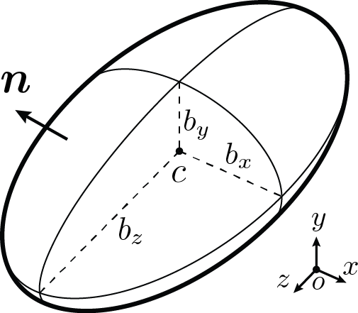
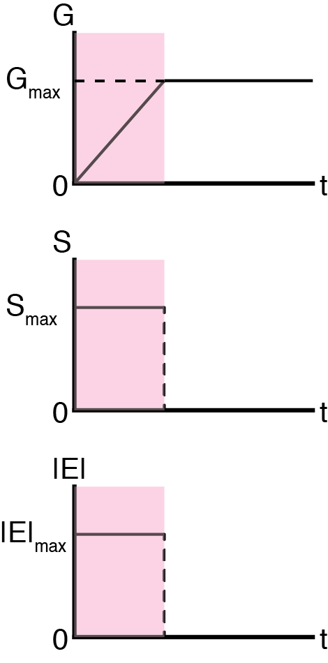
Fig. 2. Ramp-up gradient waveform. The gradient waveform has been assumed to be played-out on each three physical gradient axes in the subsequent experiments.
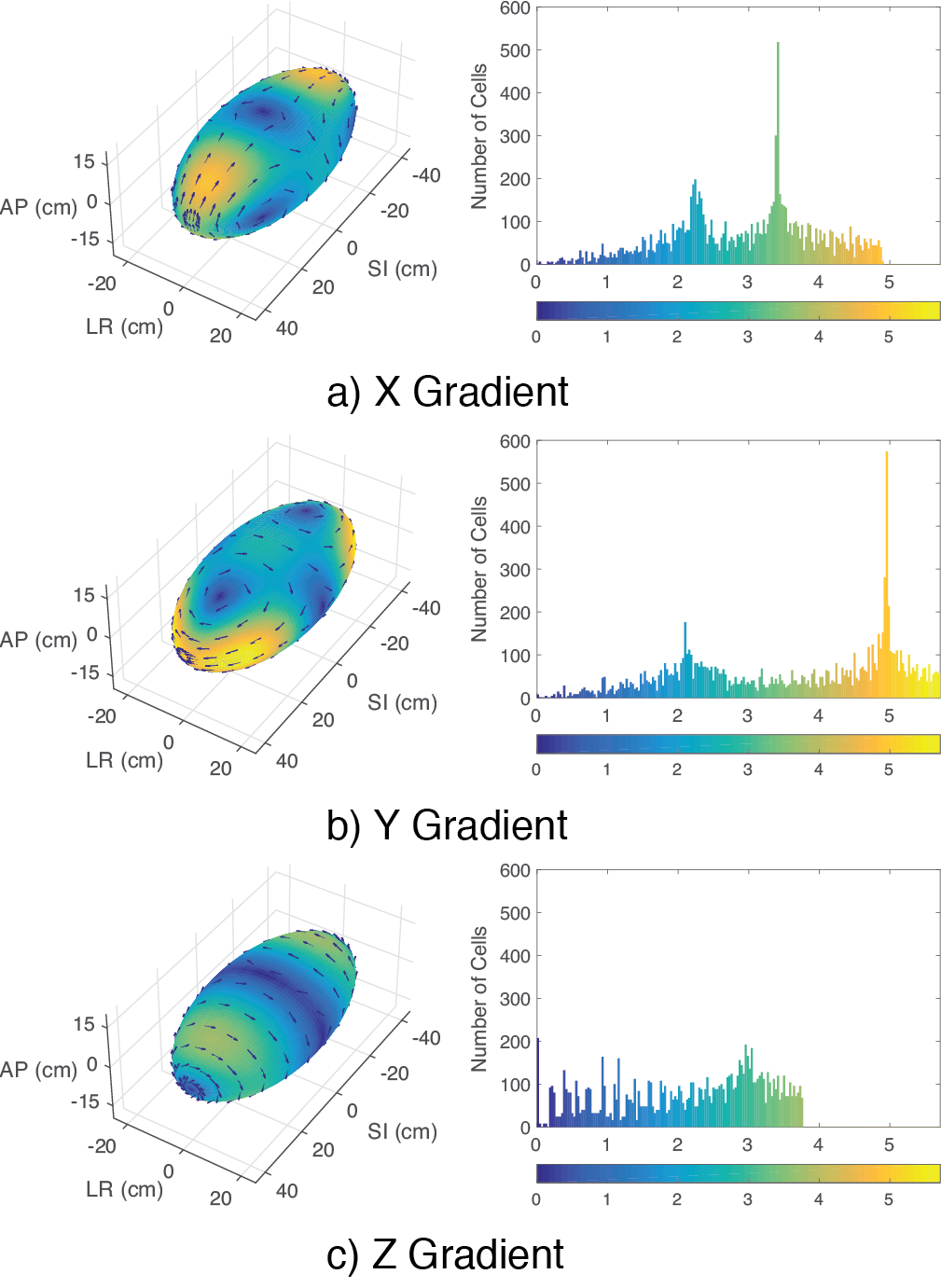
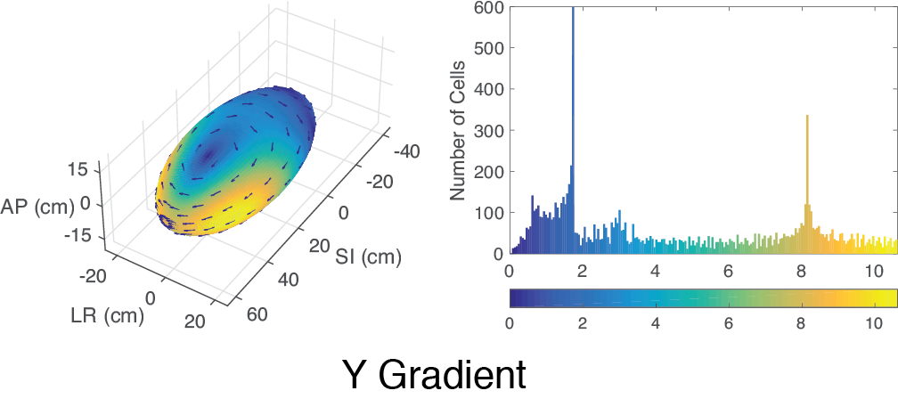
Fig. 4. Electric field induced in the ellipsoid 20cm off the isocenter (SI direction) by ramping up at 200 T/m/s on the Y gradient.