Synopsis

MR thermometry (MRT) and MR velocimetry (MRV) allow to non-invasively measure temperature and velocity fields. Therefore, they are well-suited to address medical questions; however, they can also be a valuable tool to study fluid flow and heat transfer phenomena in technical devices. Here, PRF temperature and velocity measurements were performed in a complex flow setup: a pin fin array consisting of multiple copper tubes which is frequently used in industrial processes for cooling purposes. MRV and MRT are excellent techniques to gain new insights into fundamental heat transfer phenomena and they greatly extend conventional tools for temperature and velocity measurements.

Purpose:

MR thermometry (MRT) based on proton resonance frequency (PRF)¹ and MR velocimetry (MRV)² are established methods to quantitatively monitor temperature changes (∆T) and flow, respectively. Since temperature and velocity fields are typically strongly coupled, measuring both quantities is of great interest for the engineering community, e.g. to optimize heat transfer. Compared to conventional methods such as the combination of particle image velocimetry and thermometry, MRI allows for non-invasively measuring both temperature and flow with a single experimental setup.

A few studies on MRV and MRT in fluid flows showed promising results^3,4. Recently, experiments in a counter-current double pipe heat exchanger demonstrated that MRI can accurately and precisely measure 3D velocity and temperature fields^5,6,7. In this work, the previously employed experimental approach⁵ was applied to a more complex flow setup, namely to a pin fin array consisting of multiple copper tubes which is frequently used in industrial processes for cooling purposes.

Methods:

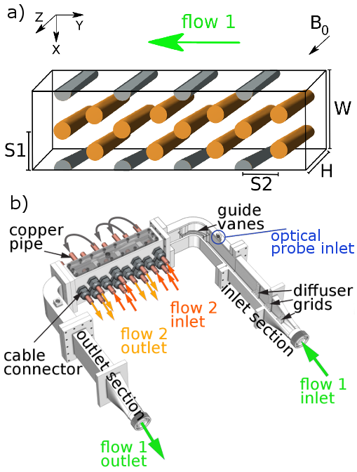
The pin fin array comprised 12 copper pipes (full pins: inner/outer diameter=10mm/12mm, length_pipes=150mm) and 8 polyamide half-cylinders (half pins) arranged in a staggered manner (Fig. 1a) forming 8 vertical rows of pins. All pins were fixed to the casing of a rectangular flow channel. The flow channel and the copper pins were connected to the flow apparatus described in reference 5. The main flow around the pins (main flow direction perpendicular to the pins’ axis) is termed ‘flow1’ (flow1=5.5l/min). The temperature of the copper pins was adjusted by an internal flow (‘flow2’) through these pipes.

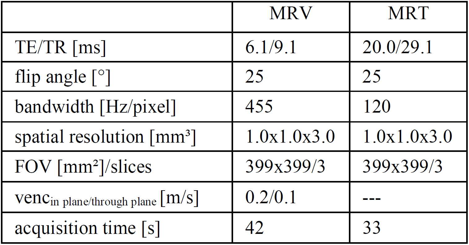
2D MRV and MRT were done at a 3T MR system (Prisma, Siemens, Erlangen, Germany) using a conventional GRE-sequence for MRV and a velocity-compensated GRE-sequence for PRF temperature mapping (imaging parameters listed in Tab. 1). Two scenarios were investigated: 1.) Homogeneous spatial temperature distribution (T_flow1=T_flow2) with a baseline acquisition at T_flow1=T_flow2=25°C and a follow-up acquisition at T_flow1=T_flow2=40°C. In total ten repetitions were acquired for both settings. 2.) Inhomogeneous spatial temperature distribution (T_flow1>T_flow2): A baseline acquisition at T_flow1=T_flow2=40°C, and a second acquisition with T_flow1=40°C and T_flow2=12°C (preventing air bubble generation at the hot surface of the copper tubes). Both acquisitions were repeated 50 times.

∆T-maps were calculated from the phase differences ∆Φ of baseline and follow-up acquisitions with the velocity-compensated GRE-sequence (∆T=∆Φ/(2π f α TE); f=123.2MHz, α_1%CuSO4=0.0097ppm/K). Reference phantoms (5%Hydroxyethylcellulose+1%CuSO₄+dist. H2O) were included to correct for field drifts (constant offset correction).

MRV was acquired 1.) with the two flows at T_flow1=40°C and T_flow2=12°C, and 2.) without any flow serving as reference scan to correct for eddy currents.

Results:

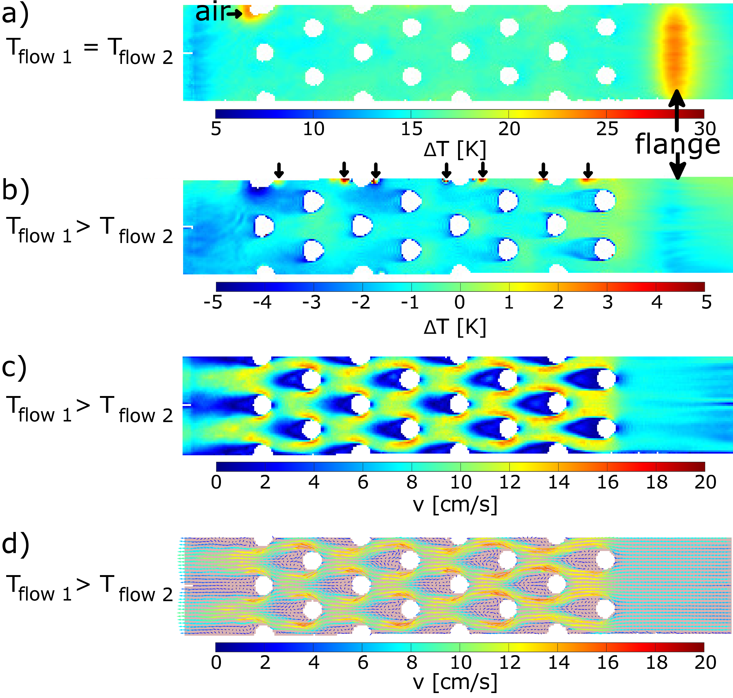
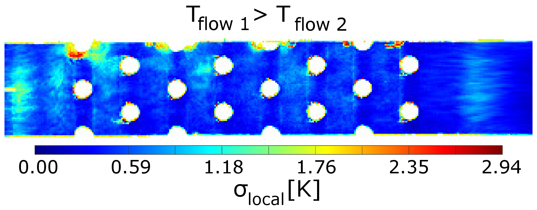
Transversal views of temperature maps (TMs) and velocity maps are shown in Fig. 2. In the case T_flow1=T_flow2 (Fig. 2a), homogeneous ∆T-maps are observed consistent with the temperature readings from a fiber optical probe (∆T_{fiber optical probe}=14.975±0.011°C). Distortions are visible at the top (air bubble) and at the inflow and outflow sections (flanges connecting the array to the bends). The case T_flow1>T_flow2 shows an inhomogeneous temperature distribution (Fig. 2b) with a ∆T decrease of about -1.6K from right to left (direction of flow1). The temperature change of flow1 between the inlet and outlet measured with fiber optical probes was -1.537±0.004K. The voxel-wise standard deviation of 50 consecutively ∆T-maps was ≲0.5K for the vast majority of voxels and thus, the temperature uncertainty was ≲0.14K (Fig. 3).

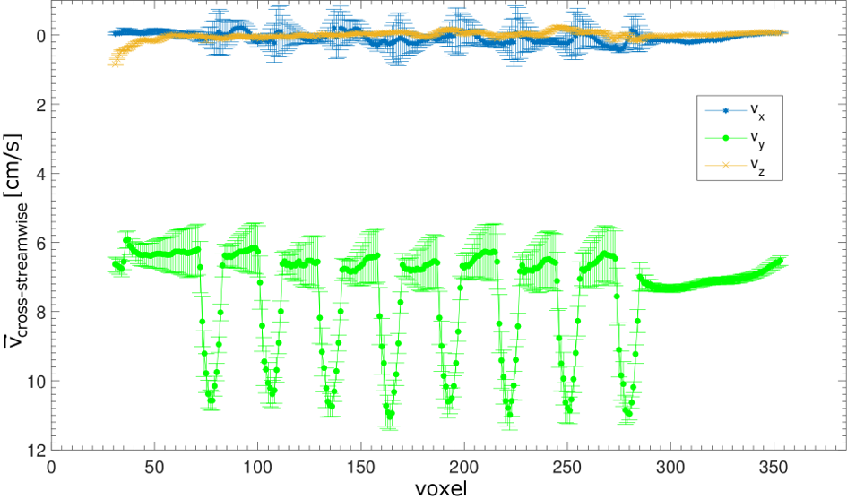
Velocity magnitude (Fig. 2c) and vector fields (Fig. 2d) show a symmetric flow pattern around the pins and ~0cm/s at the backside of the pins. The average cross-streamwise velocity v_x (parallel to the gravitational force) indicates that buoyancy forces were negligible (Fig. 4, v_x~0cm/s). The Reynolds numbers of flow1 and flow2 for the acquisition with T_flow1=40°C and T_flow2=12°C were 3000 and 7200, respectively.

Discussion:

Flow1 of the pin fin array yields a symmetric 2D velocity and temperature distribution along the x-direction since flow parallel to the pins was small and buoyancy forces were found to be negligible (case T_flow1>T_flow2). Distortions in the TMs might be explained by temperature-induced susceptibility changes and/or air bubble formation. To assess fluctuations which likely occur in the flow of the pin fin array, standard deviation maps of the TM data were calculated to locally estimate the temperature uncertainty. Field drifts are most likely the most important factor contributing to the overall uncertainty of the PRF temperature maps. Other sources of error (e.g. due to acceleration) were found to be small compared to the values measured.

The combination of MRV and MRT is a well-suited technique to gain new insights into fundamental heat transfer phenomena. MRI greatly extends conventional tools for temperature and velocity measurements in the field of flow engineering.

Acknowledgements

References

1. Rieke V and Pauly KB. MR thermometry. J Magn Reson Imaging. 2008;27(2):376-390.

2. Elkins CJ and Alley MT. Magnetic resonance velocimetry: applications of magnetic resonance imaging in the measurement of fluid motion. Exp Fluids 2007;43(6):823-858.

3. Elkins CJ, Markl M, Iyengar A, et al. Full-field velocity and temperature measurements using magnetic resonance imaging in turbulent complex internal flows. Int J Heat Fluid FL 2004;25(5):702-710.

4. Ogawa K, Tobo M, Iriguchi N, et al. Simultaneous measurement of temperature and velocity maps by inversion recovery tagging method. Magn reson imaging 2000;18(2):209-216.

5. Buchenberg WB, Wassermann F, Grundmann S, et al. Acquisition of 3D temperature distributions in fluid flow using proton resonance frequency thermometry. Magn Reson Med 2016;76(1):145–155

6. Wassermann F. Magnetic resonance imaging techniques for thermofluid applications. Dissertation 2015. Technische Universität Darmstadt

7. Buchenberg W. Development of experimental methods to measure temperature fields and velocity fields in fluid flows using Magnetic Resonance Imaging, Dissertation 2016 (submitted), Albert-Ludwigs-Universität Freiburg

8. Benhamadouche S, Howard R and Manceau R. Case 15.2. in 15th ERCOFTACSIG15/IAHR Workshop, 2011