5423
In Vivo Evaluation of a Multi-echo Pseudo-Golden Angle Stack of Stars Thermometry Method1Radiology and Imaging Sciences, University of Utah, Salt Lake City, UT, United States
Synopsis
A multi-echo pseudo-golden angle stack of stars sequence for use in free-breathing interventional procedures is evaluated in vivo with 5 healthy volunteers for use in MR thermometry in the breast. High spatial and temporal resolution (1.3 mm3, 1.43 s) is achieved through k-space filtering. PRF temperature, T2*, ρ (signal magnitude at TE = 0), respiration correction and fat/water separation are simultaneously measured. Use of a pseudo-golden angle increment allows for the removal of phase (and therefore PRF temperature) artifacts due to changing k-space sampling between reconstructed time points. k-Space sampling based phase reference library greatly improves temperature standard deviation compared to a single baseline reference.
Purpose
Radial acquisitions offer several unique advantages for proton resonance frequency (PRF) shift thermometry. Frequently sampling the k-space center provides motion robust images, as well as the ability to correct for respiration induced off resonance1. Arbitrarily high spatial and temporal resolution can be achieved by acquiring successive radial spokes separated by the golden angle and applying a sliding k-space filter, similar to the k-space weighted image contrast (KWIC) filter2, to the reconstruction3. This work investigates a pseudo-golden angle 3D multi-echo stack of stars acquisition to simultaneously measure PRF shift temperature, T2* and ρ (signal magnitude at TE = 0), correct respiration-induced off resonance, and provide water/fat separation with high spatial and temporal resolution in human breast from multiple healthy volunteers.Methods: Experiment
A 3D stack of stars spoiled GRE sequence was modified to acquire multiple echo contrasts using a bipolar readout and a pseudo-golden angle increment. The angle used, based on the ratio of two Fibanacci numbers α = (1 – 233/377)*360 ≈ 137.5066, will repeat the k-space trajectory after 377 views. Experiments were performed in 5 healthy volunteers laying prone in a Siemens 3T Prisma scanner with a breast-specific MRgFUS system4 to assess the effectiveness of this sequence and reconstruction technique in both coronal and sagittal orientations (1.3x1.3x1.3 mm, FOV = 166x166x20.8 mm, Matrix Size = 128x128x16, Flip Angle = 10, TR = 11 ms, 6 Echoes, TE = 2.46/3.75/5.04/6.33/7.62/8.91 ms, Partial Fourier: 5/8 in slice direction).Methods: Reconstruction
The slope of the phase vs TE at the center of k-space was used for respiration correction1. Data was then reconstructed using a sliding KWIC filter with 13 innermost lines, with each successive ring using the next higher Fibonacci number until 377 lines in the outermost ring. The sliding window was advanced 13 views between each reconstruction time point providing a temporal resolution of 1.43 seconds. The k-space sampling pattern was repeated after 29 reconstructed time points. Water and fat images were produced using the three point Dixon method with the first three echoes. T2*/ρ maps were calculated using linear regression of the log of the magnitude images vs TE, weighted by the magnitude M(TEj), as shown in Equation 1. $$\chi^2=\sum_{j=1}^nM_j (ln(M_j)-(a+bTE_j))^2,\quad a=ln(\rho),\quad b = \frac{-1}{T_2^*}\quad [1]$$Phase data (ψ) from each echo was combined using linear regression of the phases vs TE, weighted by the magnitude squared, as shown in Equation 2. $$\chi^2=\sum_{j=1}^nM_j^2 (\psi_j - (a+bTE_j))^2, \quad a=\psi_0, \quad b = \beta \quad [2]$$ PRF temperatures were calculated using four different methods. Method 1: The first image was used as the single reference phase for each echo independently. Method 2: A multi-baseline library was used where the reference image had the same k-space sampling pattern as the current time point for each echo independently. Method 3: The combined echo phase was used with the first image as the reference. Method 4: The combined echo phase was used with the k-space sampling pattern multi-baseline library.
Results
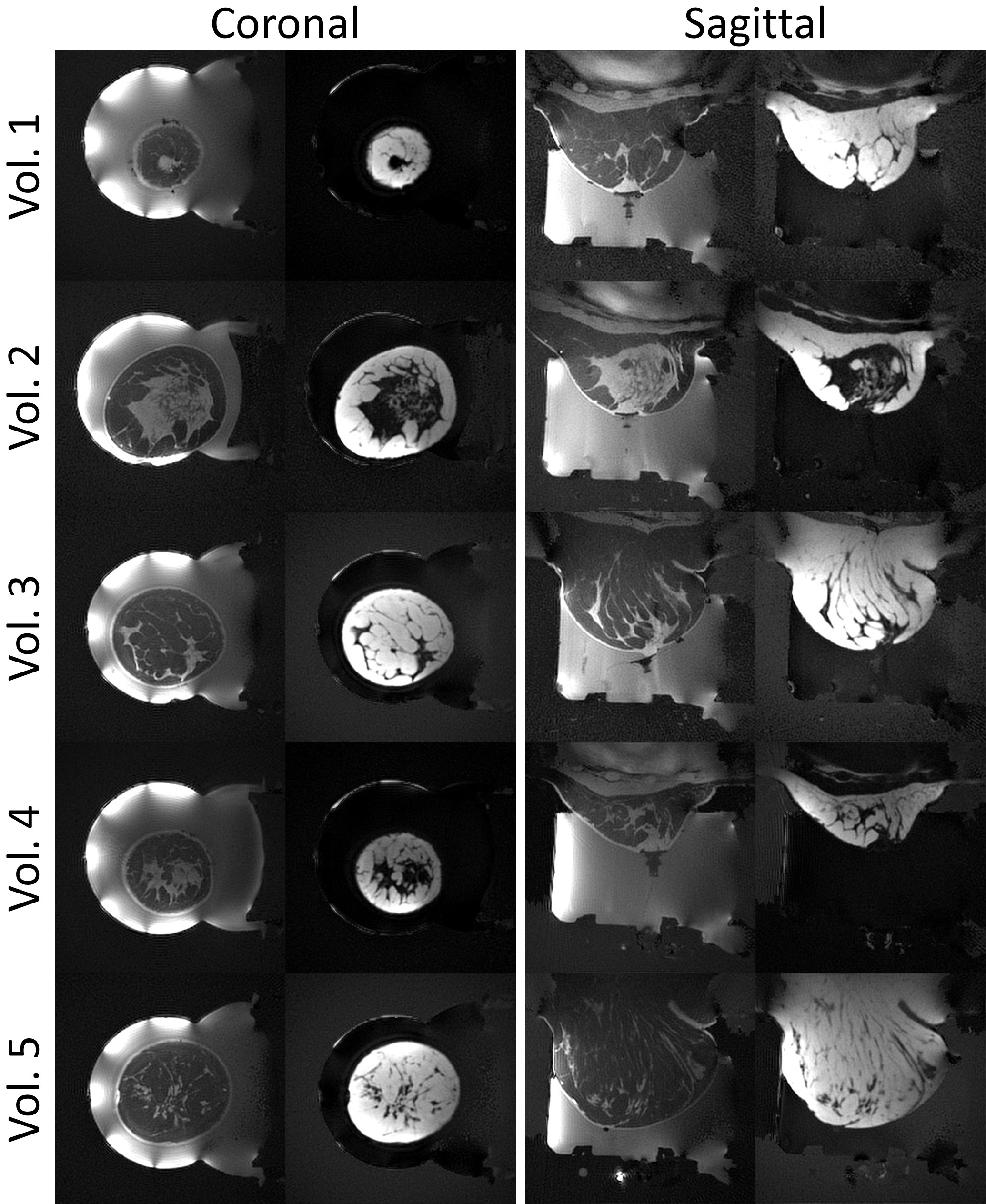
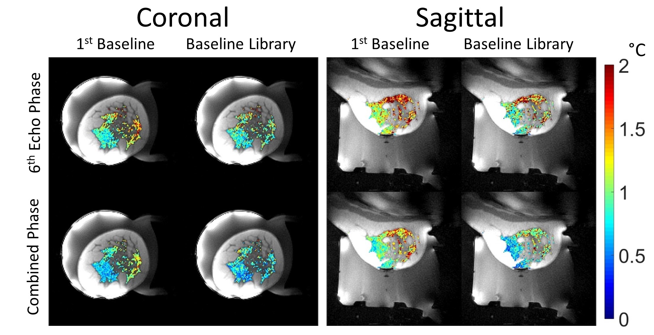
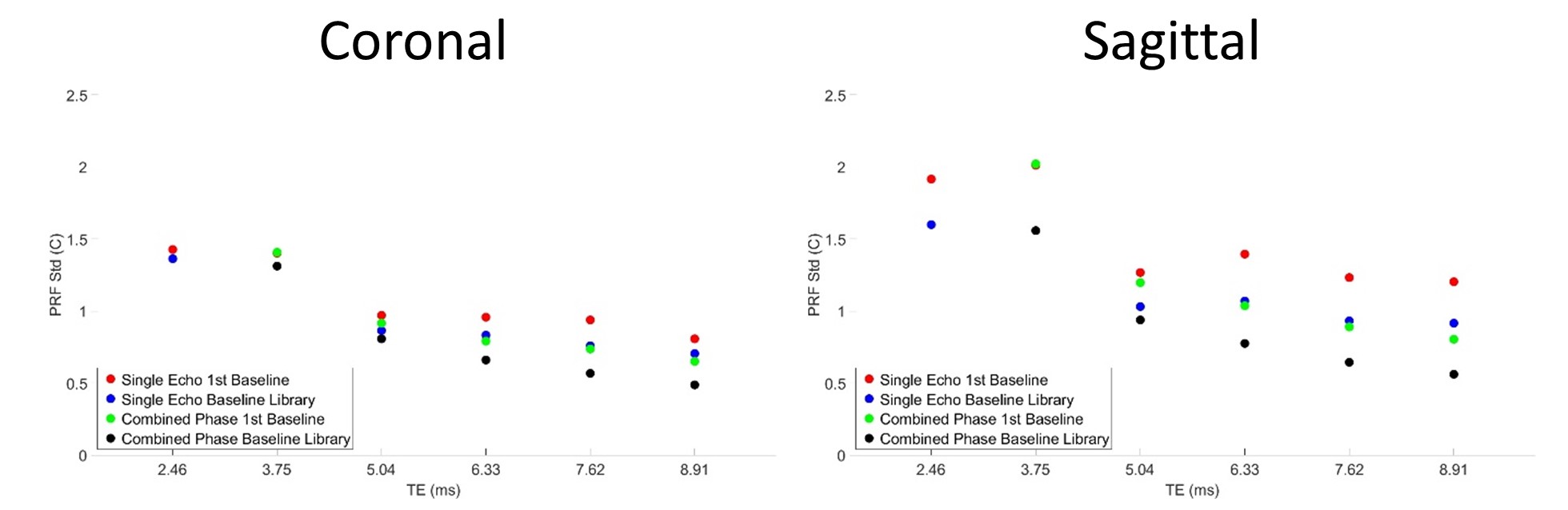
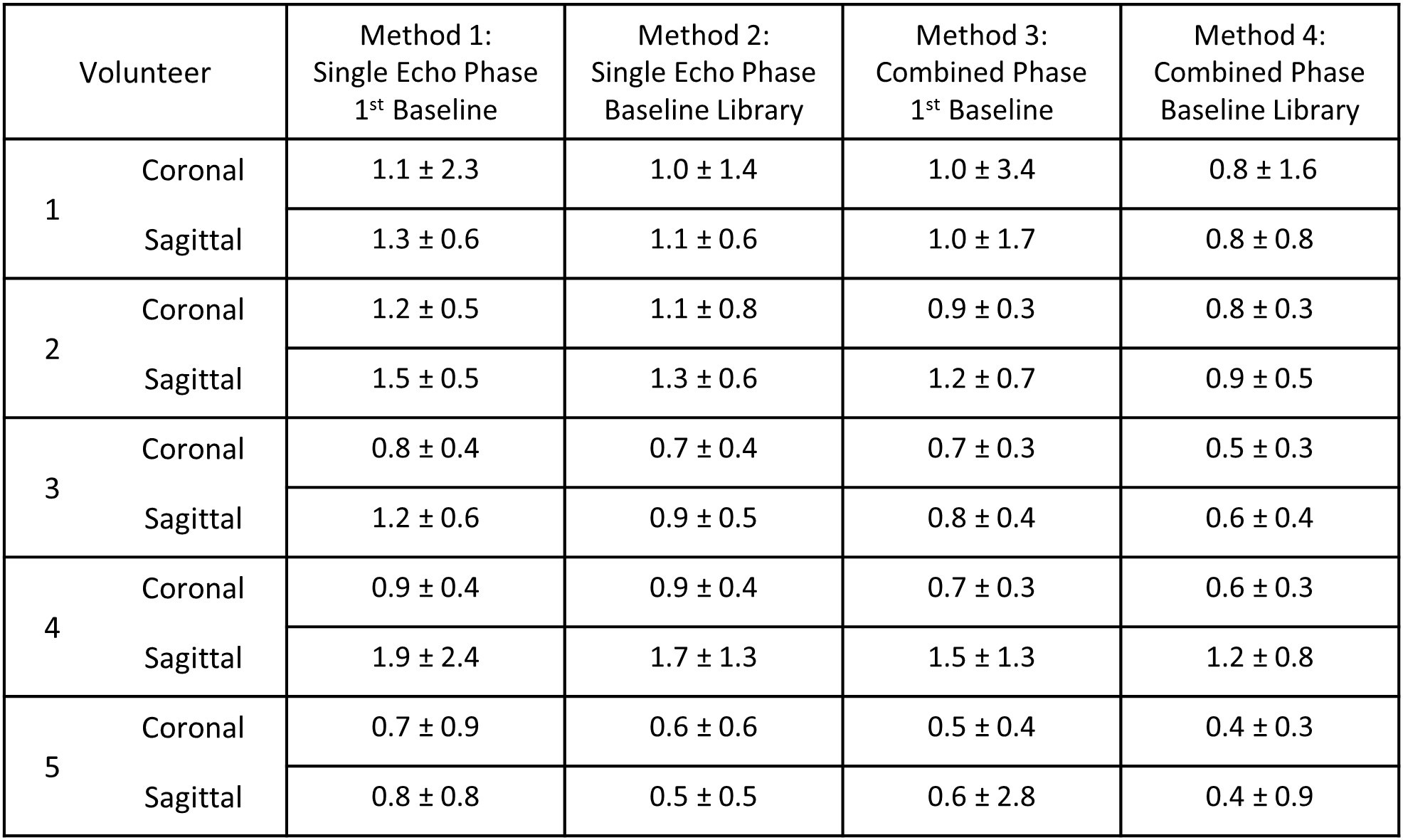
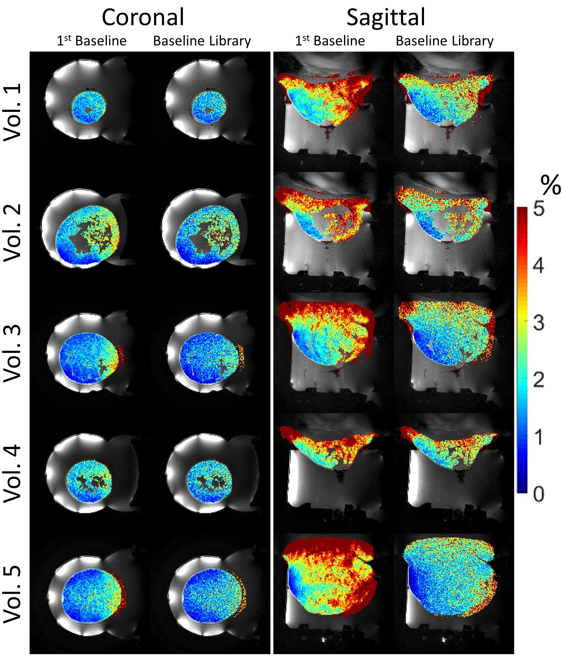
Figure 1 shows the central slice of the water and fat images produced from the sequence for each of the 5 volunteers. Figure 2 shows an example of the PRF temperature standard deviation in aqueous tissue for the 4 methods for volunteer 2. Figure 3 displays the mean PRF precision within the breast vs TE for the four methods of calculating PRF temperature change for volunteer 3. Table 1 lists the mean PRF precision within aqueous tissue in the breast for all 5 volunteers for each of the four PRF calculation methods. Figure 4 displays the precision of the initial magnitude ρ as a percent change in adipose tissue.Discussion and Conclusions
This method simultaneously creates separate water and fat images, and measures PRF temperature, T2* and ρ with a large field of view (166x166x20.8 mm), high spatial resolution (1.3 mm3) and high temporal resolution (1.43 s). The PRF precision within all 5 volunteers varied from 0.4 to 1.2 °C using the combined phase and baseline library for both coronal and sagittal orientations. The T2* and ρ measurements could be used as another possible measure of temperature change, especially in adipose tissue which does not exhibit a PRF shift with temperature5,6. All reconstructed images contain residual artifacts from regridding and KWIC undersampling which will change between reconstructed time images as the KWIC filter is advanced. For this reason, a pseudo golden angle increment was chosen to cause the residual artifacts to repeat and thus be removable in temperature difference measurements by using a baseline library. The method shown here provides promising results for this sequence and reconstruction method for use in free breathing interventional treatments.Acknowledgements
Funding Sources: NIH R01 EB013433, CA 172787References
1. Svedin BT, Payne A, & Parker DL. Respiration artifact correction in three-dimensional proton resonance frequency MR thermometry using phase navigators. Magn Reson Med. 2015;doi:10.1002/mrm.25860
2. Song HK, & Dougherty L. k-space weighted image contrast (KWIC) for contrast manipulation in projection reconstruction MRI. Magn Reson Med, 2000;44(6), 825-832.
3. Winkelmann S, Schaeffter T, Koehler T, Eggers H, & Doessel O. An optimal radial profile order based on the Golden Ratio for time-resolved MRI. IEEE Trans Med Imaging, 2007;26(1), 68-76.
4. Payne A, Merrill R, Minalga E, Vyas U, de Bever J, Todd N, Hadley R, Dumont E, Neumayer L, Christensen D, Roemer R, Parker D. Design and characterization of a laterally mounted phased-array transducer breast-specific MRgHIFU device with integrated 11-channel receiver array. Medical physics 2012;39(3):1552-1560.
5. Baron P, Ries M, Deckers R, de Greef M, et al. In vivo T2 -based MR thermometry in adipose tissue layers for high-intensity focused ultrasound near-field monitoring. Magn Reson Med, 2014;72(4), 1057-1064.
6. Rieke V, Butts Pauly K. MR thermometry. J Magn Reson Imaging 2008;27(2):376-390.
Figures