5413

Toward real-time head motion corrections in simultaneous EEG-fMRI: Convolutional neural network classification of EEG-derived motion independent components.

Chung-Ki Wong¹, Vadim Zotev¹, Raquel Phillips¹, Masaya Misaki¹, and Jerzy Bodurka^1,2,3

¹Laureate Institute for Brain Research, Tulsa, OK, United States, ²Stephenson School of Biomedical Engineering, University of Oklahoma, Norman, OK, United States, ³Center for Biomedical Engineering, University of Oklahoma, Norman, OK, United States

Synopsis

In EEG-fMRI, EEG electrodes record head motions with a high temporal resolution (EEG-motion-sensor), which can be utilized for retrospective slice-by-slice fMRI motion correction. EEG motion components derived from independent component (IC) analysis were automatically identified by the common features observed in the IC mean power spectral density, spatial projection topographic map, and signal contribution. For real-time application of the EEG-motion-sensor, pre-trained models are desirable for faster classification. We used convolutional neural network to evaluate performance of motion-IC classification model. High speed and classification accuracy were achieved on a large EEG-fMRI dataset, suggesting the possibility of real-time EEG-motion-sensor applications for fMRI.

Introduction

In simultaneous EEG-fMRI, ability of EEG cap electrodes to record and measure head motion artifacts at a high temporal resolution (EEG-motion-sensor) can be utilized to substantially remove head movements on a slice-by-slice basis in the fMRI data.^1,2 EEG motion components derived from independent component analysis (ICA)³ were automatically identified by the common features observed in the mean power spectral density, spatial projection topographic map, and signal contribution of the independent components (ICs).¹ For potential real-time application of the EEG-motion-sensor for fMRI slice-by-slice head motion corrections, pre-trained models are desirable for faster classification. Here we used convolutional neural network (ConvNet)⁴ to evaluate the performance of motion-IC classification model. In ConvNet, the convolutional layers filter local patterns of input features regardless of their positions, which improve feature recognition efficiency. Unlike the identifications based on threshold parameters, a machine learning approach benefits from a large IC dataset without the need for parameters adjustment. It also allows convenient model updates by updating the ICs database with new data.

Methods

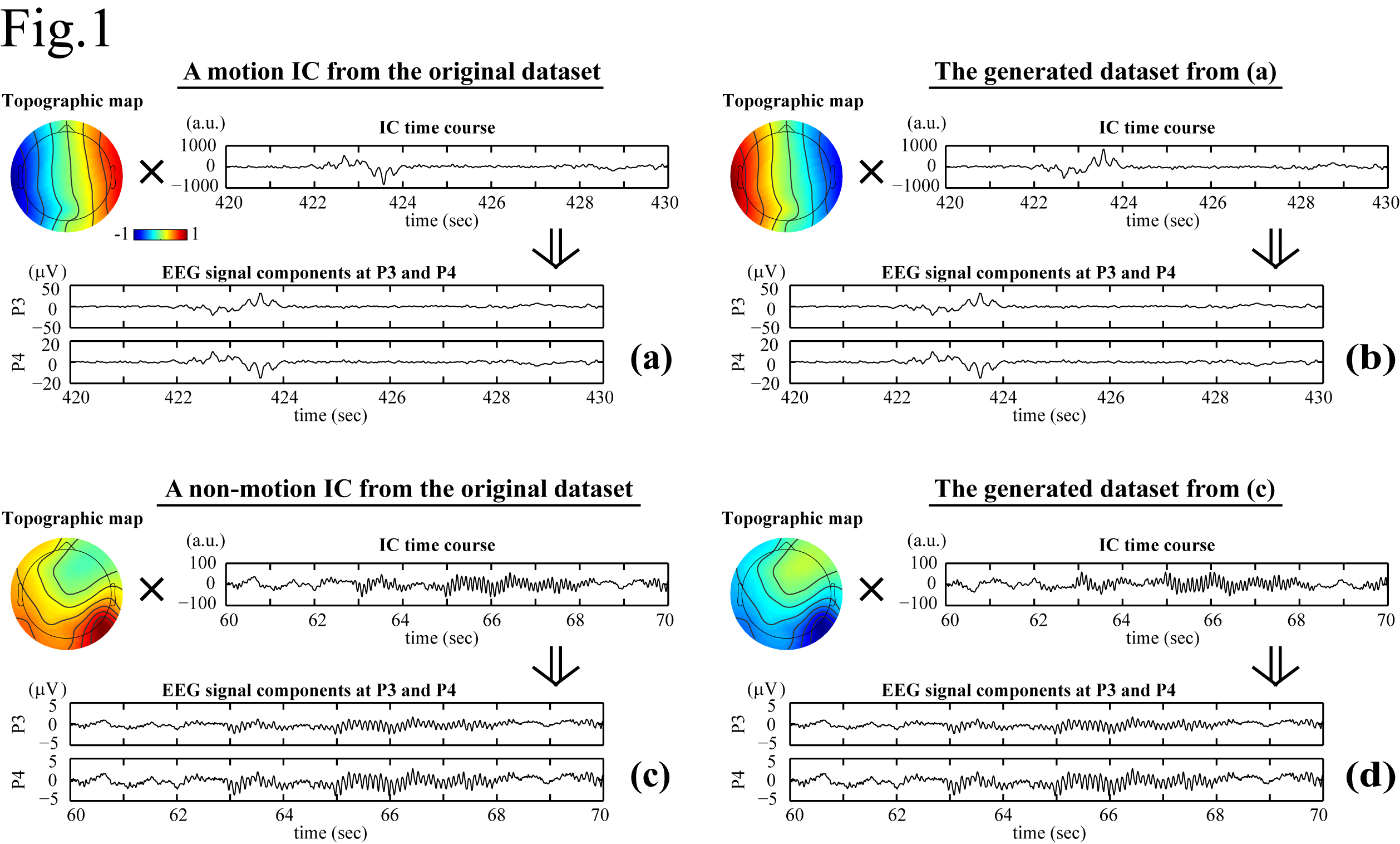
The simultaneous EEG-fMRI were conducted on a GE MR750 3T MRI with an 8ch head coil and 32ch MR-compatible EEG (Brain Products GmbH). The study included 1040 scans from 56 subjects. Each scan lasted for 526s with the first 6s removed to ensure the fMRI signal steady state. For EEG preprocessing, MRI artifacts were removed. ICA was performed on the preprocessed data to separate 31 ICs for each scan. A total of 32240 ICs were obtained. For motion-ICs classification, 92 features were used. They were 31 IC spatial projection components (A), 50 points in the normalized mean power spectral density below 12Hz, and 11 IC statistical properties:⁵ max(|IC(t)|), max(IC(t))-min(IC(t)), max(|IC'(t)|), stdev(IC(t)), skew(IC(t)), kurt(IC(t)), mean(IC(t)²)*mean(A²), mean(var(IC(τ₁))), mean(var(IC(τ₂))), mean(skew(IC(τ₁))), and mean(skew(IC(τ₂))).⁶ Here t spans the scan duration, τ₁=1s and τ₂=10s are durations of moving periods, and IC' is the IC time derivative. It is noted that simultaneous changes of the signs of A and IC do not affect the EEG signal (Fig.1). To increase the number of datasets for better classification, the number of datasets is doubled by flipping the signs of A and IC (i.e., the skewness calculations of the ICs), giving a total of 64480 datasets: 38688 for training, 12896 for cross-validation, and 12896 for testing. The train and cross-validation datasets were used for model training and optimization, and the test dataset was separated for model evaluation. In the ConvNet, two convolutional layers followed by a hidden layer and a logistic regression layer were used. The cost function was L2-regularized. The classification results were evaluated on the test dataset by accuracy (Acc), precision (P), recall (R), and F₁-score. They were compared with those calculated by support vector machine (SVM) method,^6,7,8 and 1- or 2-hidden-layer multilayer perception neural network (ML1/ML2),⁹ which were essentially the ConvNet with the convolution layers removed (ML1) or replaced by another hidden layer (ML2). The neural network calculations were carried out using Theano in Python.¹⁰

Results

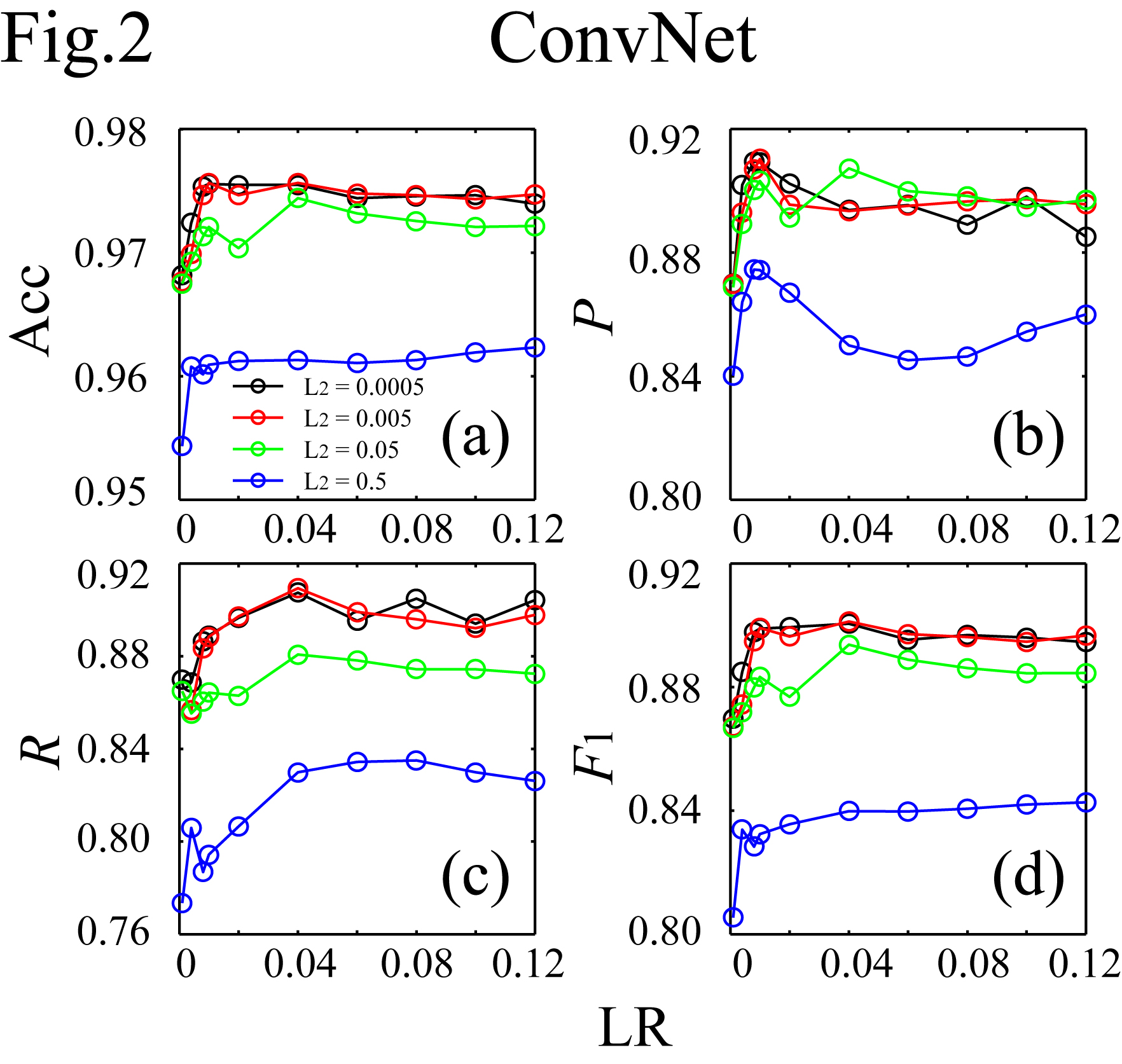
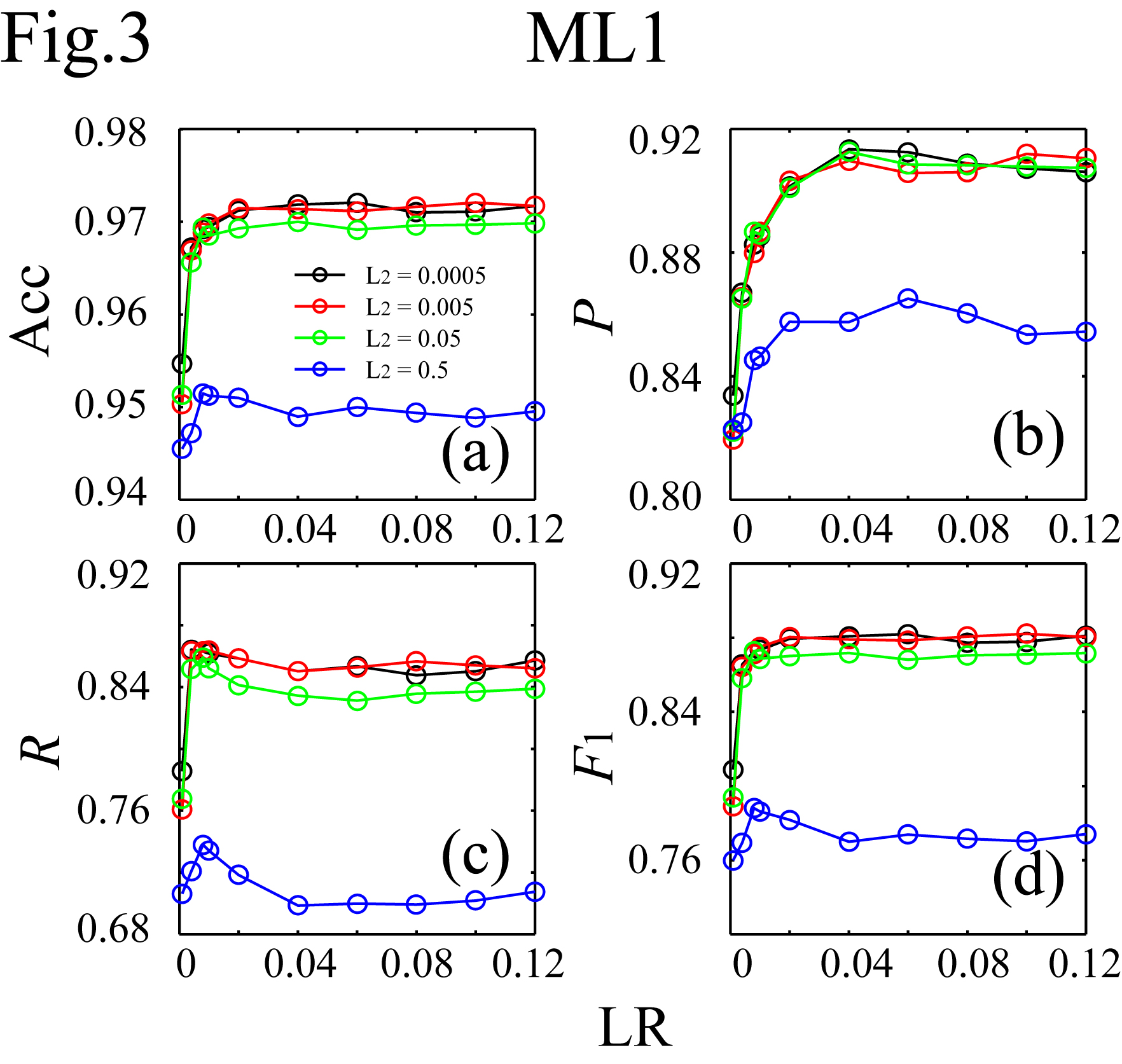
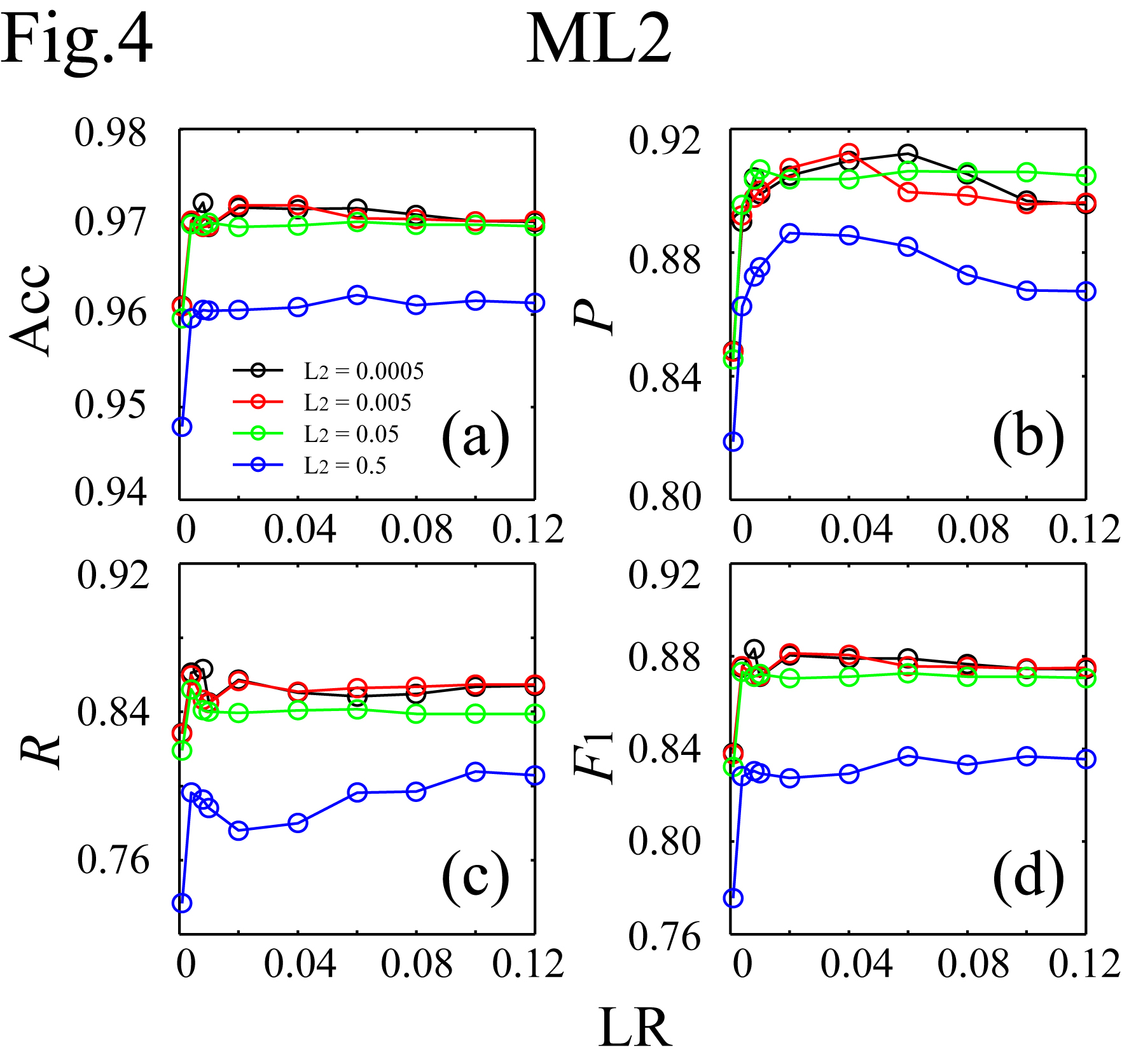
It takes about 4.5s to classify the test dataset (0.35ms/IC on average) on Intel® Xeon® workstation at 2.50GHz using 10 threads. Figs.2-4 plot (Acc,P,R,F₁) against the learning rate (LR) for different regularization parameters (L2) for ConvNet, ML1 and ML2. In the plots, (Acc,P,R,F₁) achieve (0.976,0.910,0.888,0.899), (0.972,0.912,0.854,0.882), and (0.972,0.904,0.863,0.883) for ConvNet, ML1 and ML2 respectively. The precisions of ML1 and ML2 are comparable to that of ConvNet, but the recall, and hence F₁, are significantly lower. There are two types of head motion-ICs: the spontaneous and cardioballistic motion-ICs.^1,2 When the two types of motion-ICs were classified by two separate SVM models, (Acc,P,R,F₁)_2-models=(0.967,0.876,0.851,0.863). When one model was used, (Acc,P,R,F₁)_1-model=(0.970,0.882,0.874,0.878). Among all models, ConvNet gives the highest accuracy for the motion-ICs classification.

Discussions and Summary

Motion-ICs from EEG-fMRI were classified based on a database of 64480 ICs (7612 motion-related) without presetting or adjusting threshold parameters using the convolutional neural network. The average time to classify one IC dataset is about 0.35ms. The result achieves high speed and classification accuracy (97.6%), which suggests the possibility of the EEG-motion-sensor application for real-time slice-by-slice fMRI head motion corrections.

Acknowledgements

This work is supported by DOD award W81XWH-12-1-0607.

References

1. Wong CK, Zotev V, Misaki M, et al. An automatic EEG-assisted retrospective motion correction for fMRI (aE-REMCOR). NeuroImage. 2016;129:133-147.

2. Zotev V, Yuan H, Phillips R., et al. EEG-assisted retrospective motion correction for fMRI: E-REMCOR. NeuroImage. 2012;63:698-712.

3. Bell AJ and Sejnowski TJ. An information-maximization approach to blind separation and blind deconvolution. Neural Comput. 1995;7:1129-1159.

4. LeCun Y, Bottou Y, Bengio Y, et al. Gradient-based learning applied to document recognition. Proc. IEEE 1998;86:2278-2324.

5. Winkler I. Automatic classification of artifactual ICA-components for artifact removal in EEG signals. Behavioral and Brain Functions 2011;7:30.

6. Wong CK, Zotev V, Misaki M, et al. Support vector machine classification of head motion independent components from EEG-fMRI. Proc. Org. Hum. Brain Map 2016;22:1811.

7. Cortes C. and Vapnik V. Support-vector networks. Machine Learning 1995;20:273-297.

8. Christianini N. and Shawe-Taylor J.C. An introduction to support vector machines and other kernel-based learning methods. Cambridge University Press, Cambridge, UK. 2000.

9. Christopher M Bishop. Pattern recognition and machine learning. 2006; Section 5.

10. Theano Development Team. Theano: A Python framework for fast computation of mathematical expressions. May 2016. arXiv:1605.02688 [cs.SC].

Figures

Fig.1: The topographic maps, time courses and corresponding signal components of the ICs from (a), (c) the original datasets and (b), (d) the generated datasets. The topographic map is formed by interpolating the spatial projection components (A). The datasets in (b) and (d) were generated from (a) and (c) by changing the signs of A and IC simultaneously. The resultant signal components in (b) and (d), and hence the class labels, are equivalent to those in (a) and (c).

Fig.2: The plots of (a) accuracy (Acc), (b) precision (P), (c) recall (R) and (d) F₁-score against the learning rate (LR) for different regularization parameters (L2) for ConvNet. Among the highest F₁-scores, comparable F₁ with competing P and R values are found at LR=(0.01,0.02,0.04). For a given F₁, LR=0.01 gives the highest P. For LR=0.01, the largest F₁-score is found at L2=0.005, where (Acc,P,R,F₁)=(0.976,0.910,0.888,0.899).

Fig.3: The plots of (a) accuracy (Acc), (b) precision (P), (c) recall (R) and (d) F₁-score against the learning rate (LR) for different regularization parameters (L2) for ML1. The F₁-score begins to reach the steady value 0.88 at LR=0.02. The largest F₁-score is found at (LR,L2)=(0.10,0.005), where (Acc,P,R,F₁)= (0.972,0.912,0.854,0.882).

Fig.4: The plots of (a) accuracy (Acc), (b) precision (P), (c) recall (R) and (d) F₁-score against the learning rate (LR) for different regularization parameters (L2) for ML2. The F₁-score saturates to the value 0.88 at LR=0.008. For LR=0.008, the largest F₁-score is found at L2=0.0005, where (Acc,P,R,F₁)=(0.972,0.904,0.863,0.883).

Proc. Intl. Soc. Mag. Reson. Med. 25 (2017)

5413