Purpose

To develop a more reliable functional neuroimaging technique to achieve high-resolution spatiotemporal mapping of brain activities.

Method

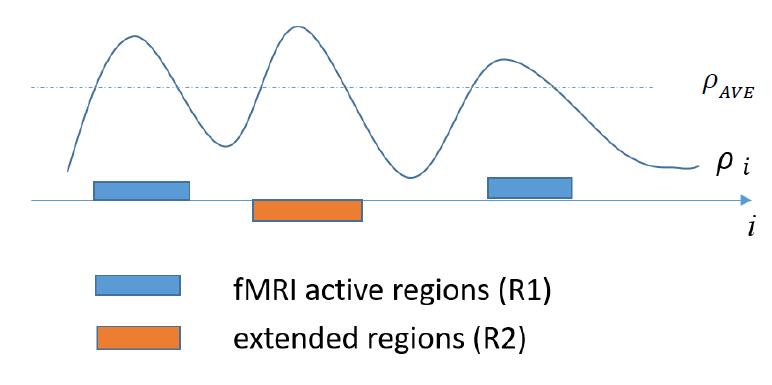
The forward solution of EEG/MEG can be expressed in a simple vector notation: $$x=Ls+n $$where x is the vector of electric/magnetic recordings, L is the gain matrix, s is the vector of dipole strengths, and n is the vector of noise at each electrode or sensor. The optimal linear inverse operator G can be written as: $$G=RL^{T}(LRL^{T}+C)^{-1} $$where C is the noise covariance matrix and R is the source covariance matrix1. In the proposed method modified fMRI-weighted minimum-norm estimation (mfMNE), the matrix R is determined using both the estimated neural activity (i.e. $$$w_{e}$$$ ) and vascular activity measured by fMRI (i.e. $$$w_{f}$$$ ): $$R=w_{e}w_{f} \quad $$ $$$w_{e}$$$ can be constructed by taking its diagonal elements to be the minimum-norm estimation (MNE) solution as follows: $$w_{e}=\begin{bmatrix}s_{1} & \cdots & 0\\ \vdots & \ddots &\vdots\\ 0 & \cdots & s_{n}\end{bmatrix} $$ where $$$s_{n}$$$ represent the estimated dipole strength at location n. The estimated source strength $$$\hat{s}_{i}$$$ at each location i can be written as: $$\hat{s}_{i}\left(t\right)=G_{i}x\left(t\right) $$ $$=G_{i}\left(Ls\left(t\right)+n\left(t\right)\right) $$ $$=\sum_{j1}\left(G_{i}L_{j1}\right)s_{j1}(t)+\sum_{j2}\left(G_{i}L_{j2}\right)s_{j2}\left(t\right)+\cdots+\sum_{jk}\left(G_{i}L_{jk}\right)s_{jk}\left(t\right)+G_{i}n(t) $$A $$$\rho_{i}$$$ metric is defined similar to the ‘crosstalk’ metric as follows: $$\rho_{i}=\frac{\sum_{t1}\hat{s_{i}}}{\sum_{t}\hat{s_{i}}}=\frac{\sum_{t1}\sum_{j1}(G_{i}L_{j1})s_{j1}(t1)}{\sum_{t}\hat{s_{i}}} $$ The metric $$$\rho_{i}$$$ describes how well the estimated curve represents the simulated curve for activation occurring at location i during t1. An average of $$$\rho_{i}$$$ ($$$\rho_{AVE}$$$) is calculated for the cortical vertices that belong to the given fMRI activation regions (R1) in Fig.1. The source points outside the given fMRI activation regions, of which the integrated source intensities exceed $$$\rho_{AVE}$$$, are included in the new prior activation regions (R2). The diagonal elements of $$$w_{f}$$$ corresponding to fMRI-visible areas of activation (R1+ R2) are set to 1. Those locations that are not visible by fMRI (missing locations) are set to 0.1. The Monte Carlo simulation was conducted based on a realistic-geometry boundary element method (BEM) model. The mfMNE, MNE and dynamic Statistical Parametric Mapping (dSPM) models were compared using 200 groups of simulated data, including two scenarios: no silent activity and silent vascular activity. The visual stimulation experiment included two separate sessions with the identical visual stimuli for the EEG and fMRI data collection respectively. The stimulation was a rectangular checkerboard within the lower left quadrant of the visual field. The checkerboard was reversed at 2Hz. In the fMRI experiment, the stimuli were presented in eight 30-second blocks separated by nine 30-second resting blocks without stimulation. In the EEG experiment, the visual stimuli were presented for 15-25 seconds, with six-second breaks in between2. The anatomical MRI and fMRI data were collected on a MAGNETOM Prisma 3T MR system (Siemens, Erlangen, Germany). The whole-head T1-weighted MR images (matrix size=256×224, slice thickness=1 mm) were acquired with a MPRAGE sequence (TR/TE=2530ms/2.98ms). The T2*-weighted fMRI data were acquired using a prototype simultaneous multi-slice sequence (TR=2000ms, TE=30ms, number of slices=64, spatial resolution= 2mm x 2mm x 2mm, slice acceleration factor =2). The EEG signals were collected from a BrainAmp MR 64 plus system (BrainProducts, Gilching, Germany) with a 5000 Hz sampling rate.

Results

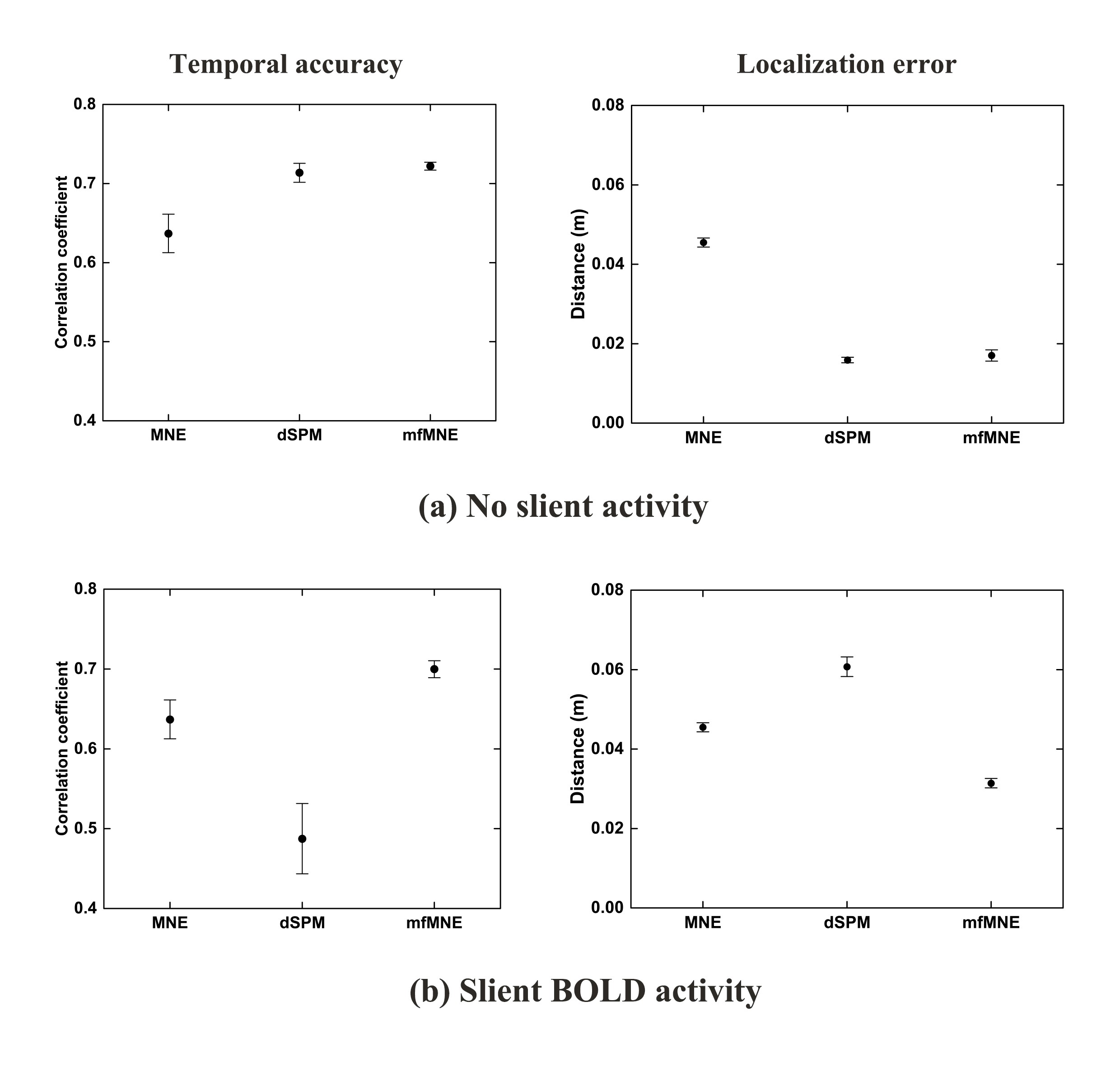
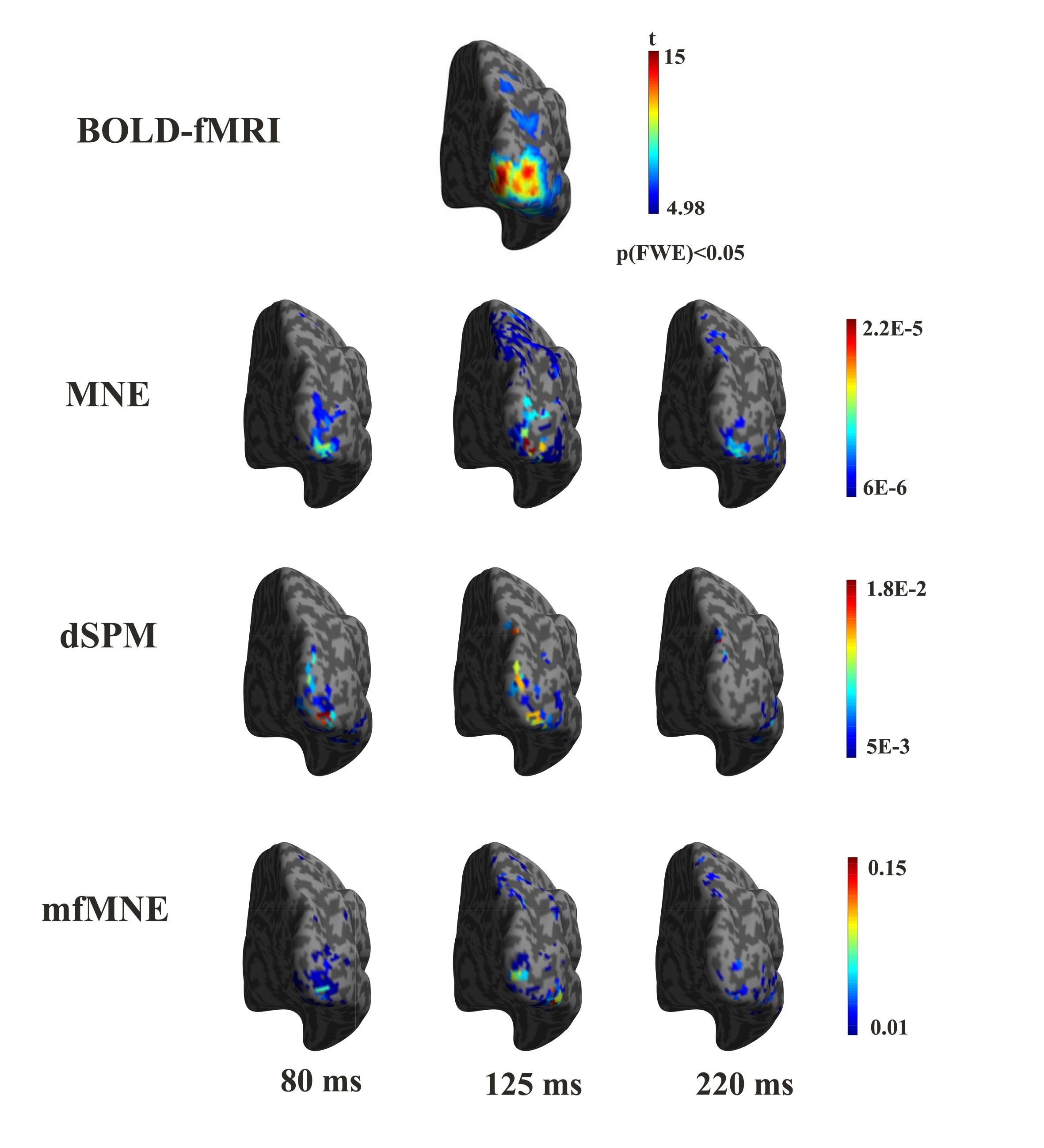
When comparing different estimation models, both the temporal and spatial properties of the simulation results were evaluated. The dSPM and mfMNE models achieved higher detection accuracy for regions, exhibiting both neural and vascular activities than MNE (Fig. 2a). When regions exhibited neural activity, but no vascular activity, the mfMNE resulted in the most accurate imaging results among all 3 algorithms (Fig. 2b). The activated cortical areas at the contralateral hemisphere were revealed in the fMRI activation map (row one in Fig. 3). The following three rows of Fig. 3 show the reconstructed contralateral CCD distribution using the three models. From the CCD images reconstructed by using the mfMNE, the dorsal pathway was seen gradually extending from lower tier to high-tier visual areas, which was generally in agreement with the well-known organization of the visual system.

Discussion

The proposed mfMNE method has two principal advancements. First, fMRI priors are modified by extending the fMRI activation regions based on the conventional EEG source imaging. Second, the mfMNE method uses both the estimated neural activity and the vascular activity measured by fMRI to estimates the source covariance matrices. Our method depends on the initialization. MNE estimate is a reasonable choice for $$$w_{e}$$$ . The results have demonstrated that the proposed method is capable of handling the mismatches between fMRI activations and EEG source activities.

Conclusion

The proposed mfMNE method estimates the source covariance matrices from both fMRI and EEG data, which provides more accurate current estimates as demonstrated by both simulated and experimental results.

Acknowledgements

No acknowledgement found.