5398
Correcting motion-affected gradient artifacts in EEG-fMRI: a modeling approach1Department of Radiology, Medical Physics, University Medical Center Freiburg, Freiburg, Germany
Synopsis
Simultaneous acquisition of electroencephalography (EEG) and functional magnetic resonance imaging (fMRI) is extensively applied for brain mapping due to the high temporal resolution of EEG and high spatial resolution of fMRI. But gradient artifacts on the EEG cannot be optimally corrected in the presence of abrupt head movements. In this work, we demonstrate a method to model motion-related gradient artifacts. Thus we obtain not only an improvement in gradient artifact correction, but also infer motion information directly from the EEG.
Purpose
In EEG-fMRI, the artefacts caused by the imaging gradients on the EEG are usually removed by averaged artifact subtraction (AAS)[1], which averages epochs of data in the time domain to form a subtraction template, assuming that the artefacts remain the same while EEG is uncorrelated across fMRI repetition times. However, the template will be distorted when there is sudden motion[2],[3]. Because of the induced potentials and the altered shape of induced gradient artifacts, a sliding-window averaged template cannot adapt to this salient change. Modeling such motion-related changes is possible, although this requires highly accurate motion measurements using specialized equipment[3]. Here we present a modeling approach that can extract motion-related modulations directly from the EEG, yielding a better reduction of gradient artifacts. Moreover, the shape of the calculated motion is very similar to measurements provided by a motion-tracking camera, thus offering motion information without requiring additional equipment.Methods
Simultaneous EEG-fMRI data were acquired in 8 epilepsy datasets at the Epilepsy Center of the University Medical Center Freiburg. FMRI had been acquired on a Siemens Prisma 3T scanner with a 3D MR-Encephalography (MREG) sequence[4] (TR=100 ms, TE=36 ms, 3D matrix size 64x64x50, voxel size 3x3x3 mm3, 30-minute acquisition time), while EEG was sampled at a rate of 5000 Hz and filtered between 0.016-250 Hz using a 64-channel MR-compatible system (BrainProducts, Germany). The EEG clock was synchronized to the 10 MHz scanner clock. Motion was recorded during the experiment with a MR-compatible optical camera (Metria Innovation, Milwaukee, USA).
According to Faraday’s law, the gradient artefacts can be expressed as:
$$S_{grad}\propto d\bf B \it /dt \approx d\bf g\it /dt \cdot \bf x$$
where x here is a 3-dimensional vector of the EEG wire loop position and g is a 3-dimensional vector of the time-dependent magnetic field gradients.
In reality, the recorded data E is acquired after filtering,
$$E = (S_{eeg}+ S_{grad})\otimes h$$
where h is the impulse response of the anti-aliasing filter of the EEG system. As we know the filter h as well as the gradient waveforms g of the fMRI sequence, it is easy to solve the equation
$$E=(d\bf g\it /dt \cdot \bf x) \otimes \it h =(d\bf g\it /dt \otimes h )\cdot \bf x$$
assuming a constant x within each epoch, resulting in an estimate of the position x at each TR by linear least squares. In practice, this does not result in a perfect fit due to effects not modeled in h (e.g. eddy currents). Consequently, we then fix the roughly fitted positions x and estimate a new filter h by Wiener deconvolution. This process is then iterated multiple times, alternatively fitting x and h, until convergence. Following the subtraction of the filtered and modulated gradient waveforms, AAS is then applied to remove any residual artifacts.
Result/discussion
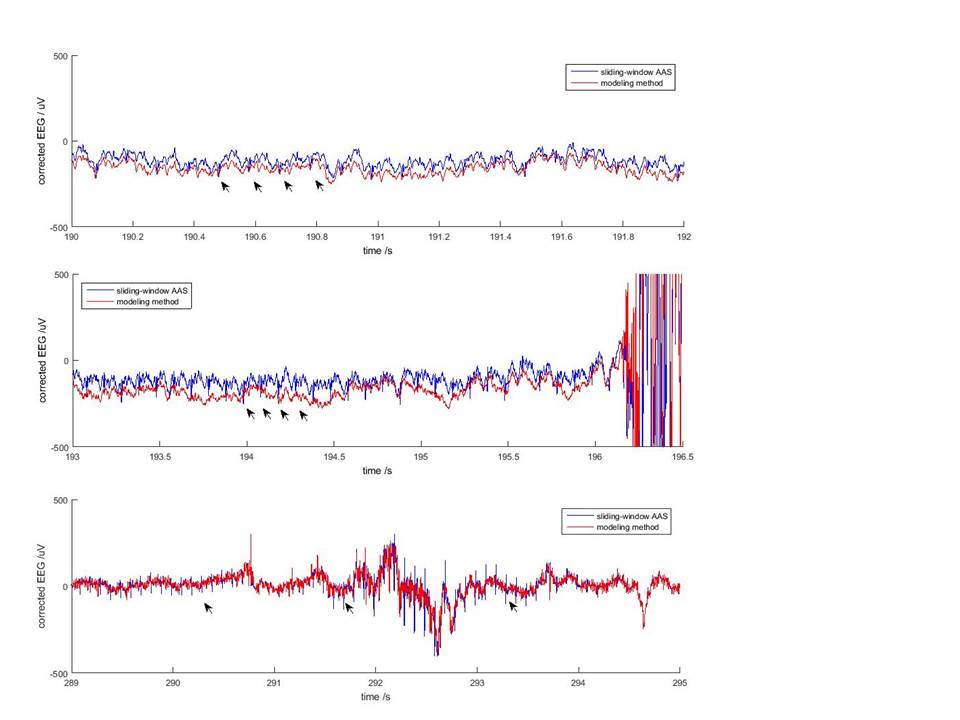
The modeling method showed a better reduction of gradient artifacts in all subjects. Fig.1 shows some examples from every subject in the vicinity of sudden motion events, where standard AAS is known to fail.
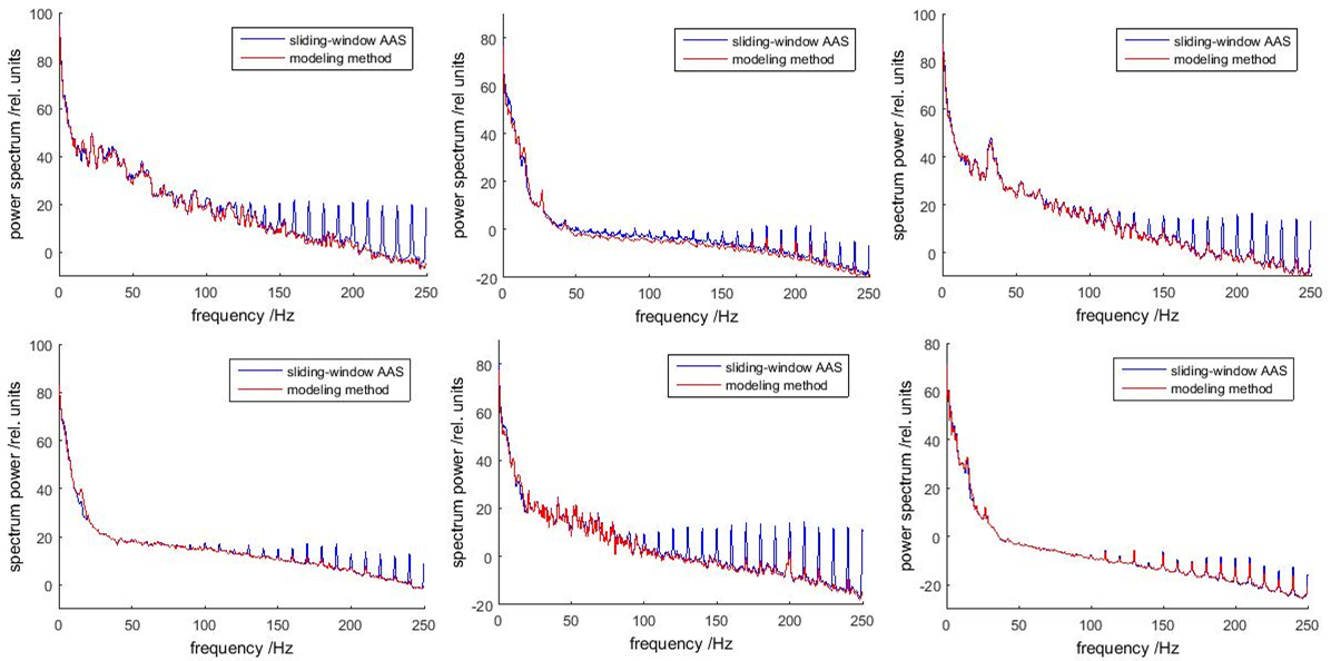
Fig.2 shows EEG spectral density from all subjects, averaged across all channels. The modeling method resulted in a better reduction of gradient noise (spectral peaks around harmonics of 1/TR = 10 Hz) without harming the underlying true signal (spectral power at other frequencies).
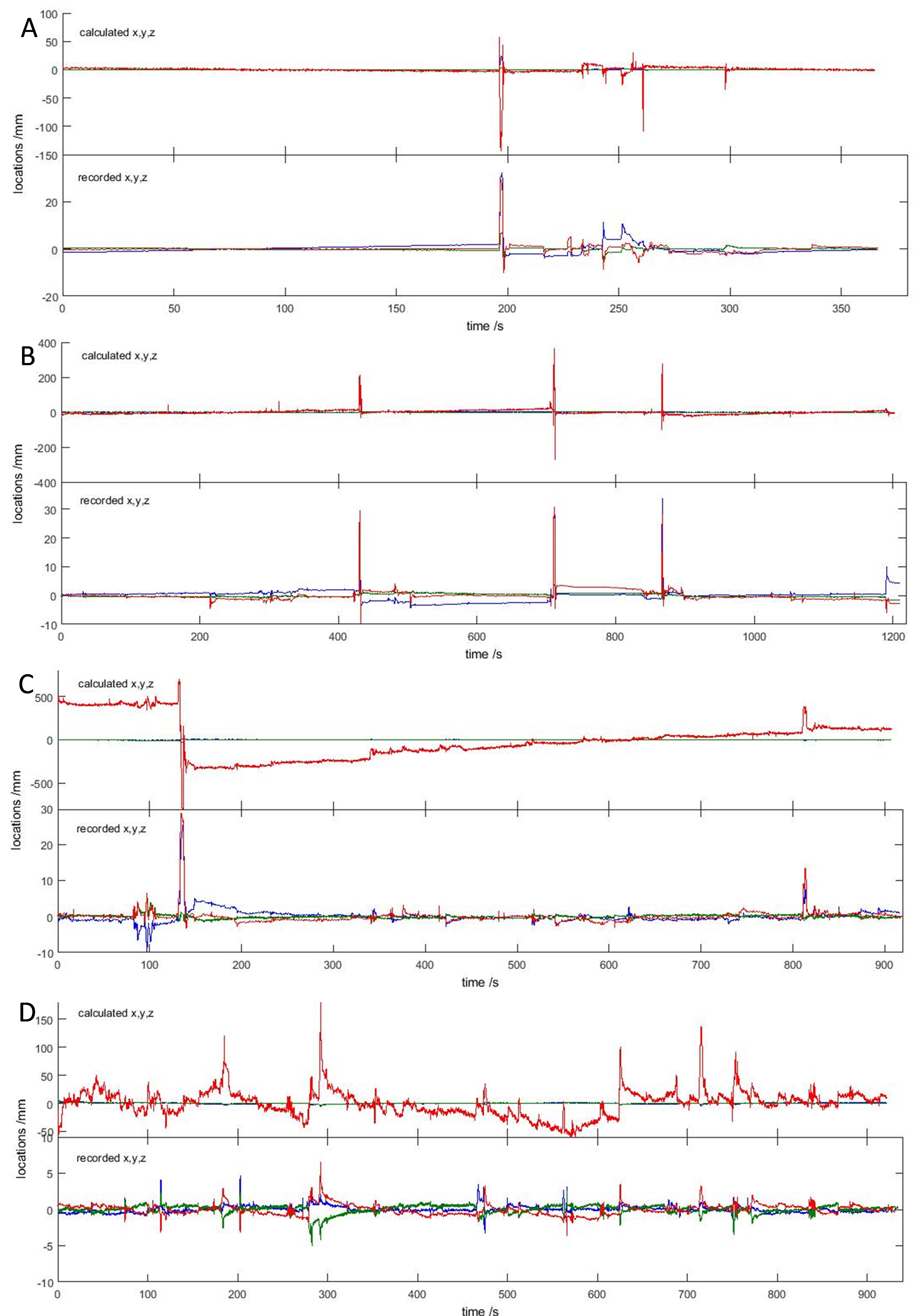
Moreover, the estimated position vector x shows great similarity with the head position measured by optical tracking (Fig.3), although we do not expect an exact match, since the estimated positions are a complex function of spatial location and orientation with respect to the magnetic field. Nevertheless, the estimated positions can successfully attenuate motion-related gradient artifacts.
Conclusion
The modeled motion-related gradient waveforms can greatly reduce the gradient artifacts that would otherwise remain after the application of sliding-window AAS, as assessed by visual inspection of EEG time courses and quantified by spectral densities. The method also allows the accurate estimation of motion information consistent with measured positions by an optical tracking camera.Acknowledgements
This work was supported by the grant He 1875/28-1 and the cluster of excellence EXC-1086 “Brain Links-Brain Tools” from the German Research Foundation (DFG), the China Scholarship Council (CSC), and the Stiftung Familie Klee.References
[1] Allen PJ, et al, (2000), ‘A method for removing imaging artifact from continuous EEG recorded during functional MRI’, Neuroimage, vol. 12, no.2, pp. 2309.
[2] M. Moosmann et al, (2009), “Realignment parameter-informed artefact correction for simultaneous EEG-fMRI recordings,” NeuroImage, vol. 45, no. 4, pp. 1144–1150.
[3] P. LeVan, et al, (2016), "EEG-fMRI Gradient Artifact Correction by Multiple Motion-Related Templates," IEEE Transactions on Biomedical Engineering, vol.PP, no.99, pp.1-1.
[4] J. Assländer, et al, (2013), “Single shot whole brain imaging using spherical stack of spirals trajectories,” NeuroImage, vol. 73, pp. 59–70.
Figures