5344
Confound Suppression in Resting State fMRI using Sliding Windows and Running Mean1Neurology, University of New Mexico, Albuquerque, NM, United States, 2Physics and Astronomy, University of New Mexico, 3Electrical Engineering, University of New Mexico
Synopsis
We analytically investigate the characteristics of a recently developed sliding window methodology designed for real time analysis of resting state connectivity. The suppression of various types of confounds is investigated both in this analytical framework and numerically. It is shown that this methodology not only acts as a high pass filter and denoiser, but behaves as a model free despiking and confound suppression tool.
Purpose
Seed-based resting-state fMRI analysis typically requires regression of movement effects and signal fluctuations in CSF/white matter to minimize false connectivity1,2. In this study we present an analytical, numerical, and experimental characterization of the recently developed windowed seed based connectivity analysis (wSCA) methodology3. This technique utilizes a running mean of sliding window correlations and has been shown to clean up resting state connectivity maps in vivo. We find that wSCA not only acts as a high pass filter and denoiser, but also as a model free despiking tool, limiting the effects of spurious correlations due to a variety of artifacts.
Theory
The following equations show correlations for the simple cases of spikes in a single time-course (Eq.1) and both time-courses (Eq.2):
$$r_{1spike} = \frac{N\sum xy - \sum x\sum y+n(Nsy_{i}-s\sum y)}{\sqrt{\bigg{(}N\sum x^{2}-\big{(}\sum x \big{)}^{2}+n(N-1)s^{2}+2ns(Nx_{i}-\sum x)\bigg{)}\bigg{(}N\sum y^{2}-\big{(}\sum y \big{)}^{2}\bigg{)}}} \quad [1]$$
$$r_{2spike} = \frac{N\sum xy-\sum x\sum y+n(N-1)s^{2}+ns(Nx_{i}+Ny_{i}-\sum x- \sum y)}{\sqrt{\bigg{(}N\sum x^{2}-\big{(}\sum x \big{)}^{2}+n(N-1)s^{2}+2ns(Nx_{i}-\sum x)\bigg{)}\bigg{(}N\sum y^{2}-\big{(}\sum y \big{)}^{2}+n(N-1)s^{2}+2ns(Ny_{i}-\sum y)\bigg{)}}} \quad [2]$$
where x and y are the time-courses being correlated, N is the number of time points, w is the window width, s is the spike amplitude, and n is the number of spikes. Equation 3 shows how wSCA modifies these correlations:
$$r_{wSCA}=\frac{1}{N-w+1}\sum_{1}^{N-2w+1}\sigma + \frac{n}{N-w+1}\sum_{1}^{w}r_{spike} \quad [3]$$
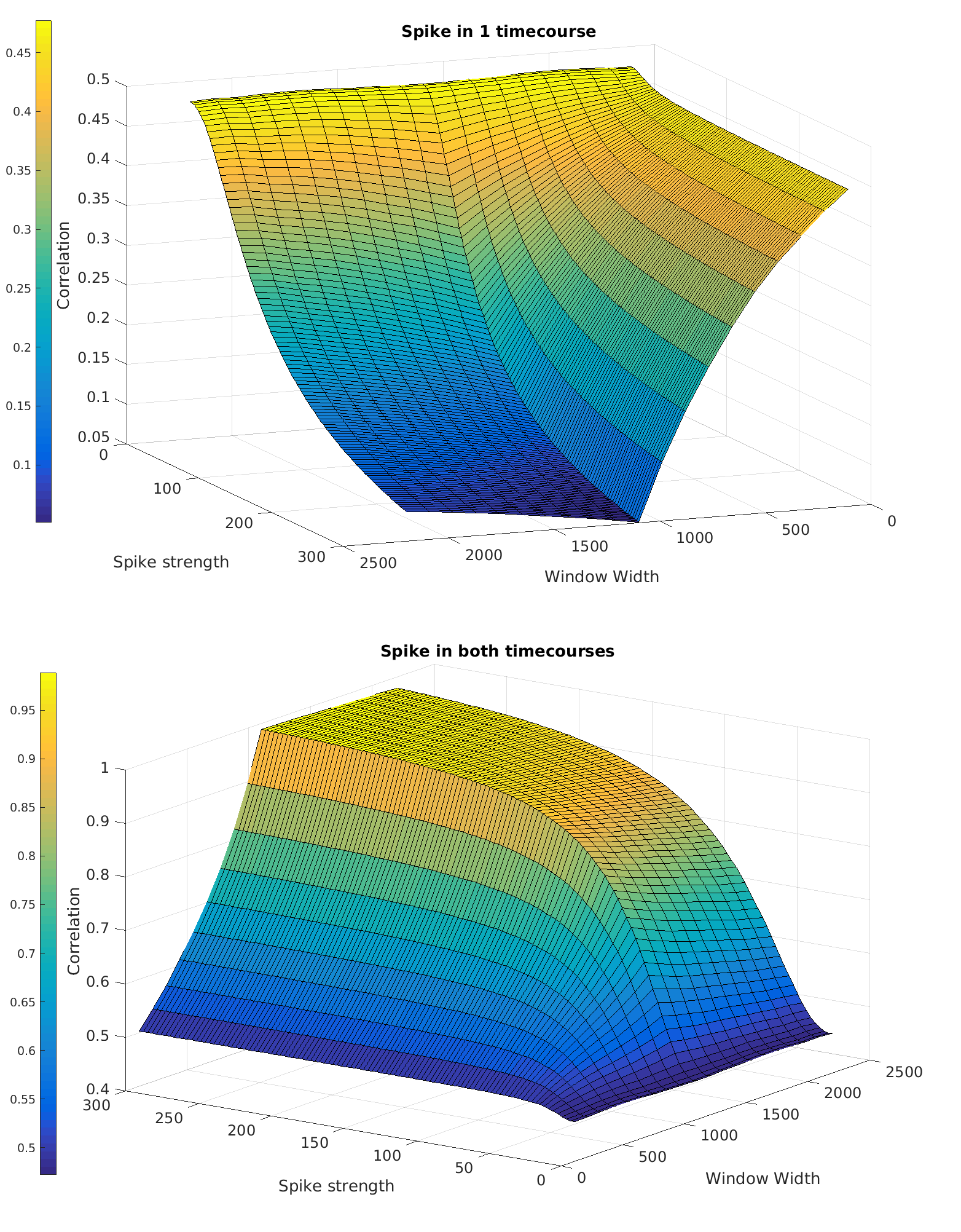
where σ is the correlation without confounds. Fig.1 shows how Eq.3 behaves analytically with varying w and s. For spike amplitude approaching zero, there is little difference between correlations with various window widths, including standard seed-based approaches (w=N). As spike strength increases, wSCA displays reduced changes in measured correlations.
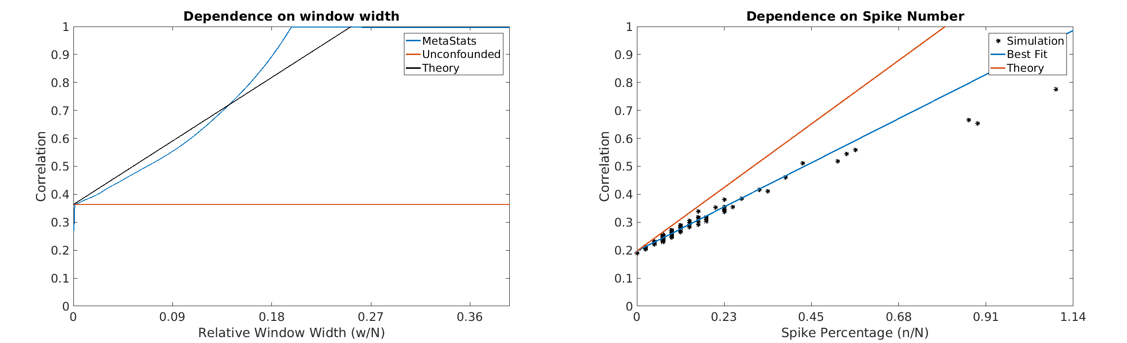
In order to further characterize the behavior of this methodology, we take the limit of Eq.3 for large spikes in both time-courses, and small values of w/N:
$$\lim_{\frac{w}{N}\to 0;s\to\infty} r_{wSCA} = \sigma + \frac{nw}{N} \quad [4]$$
In these limits, the over/under-estimation of the correlation due to the spikes decreases linearly with window width and spike number. This behavior is further explored numerically in the following section.
Methods
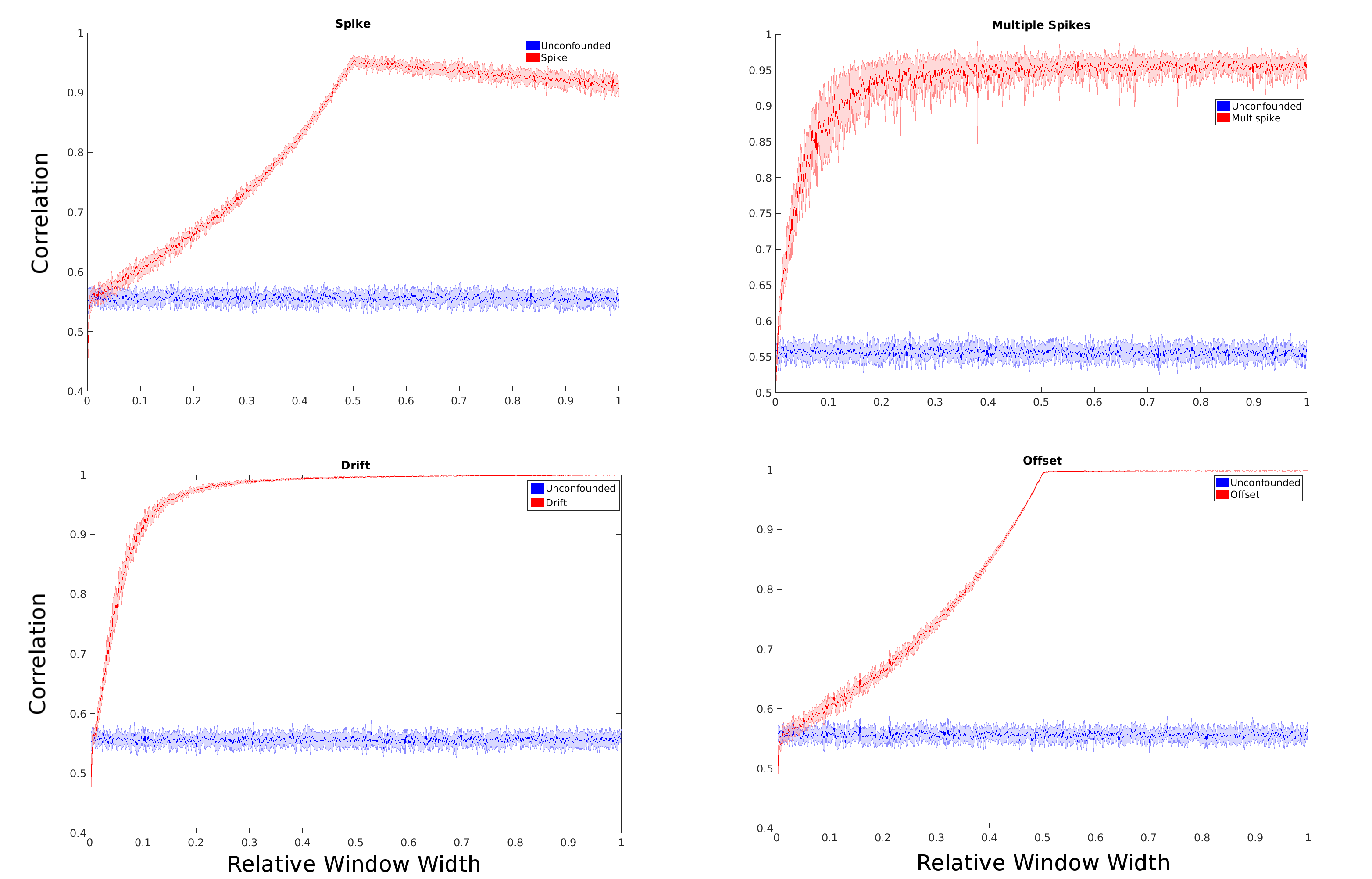
Confound suppression was characterized for a 2-node network using the model in Fig.2. Random signals (variance=1, mean=0) were generated, filtered using a simple lowpass filter, and mixed in order to induce a known correlation. Noise and confounds were added to assess the viability of different methods for reproducing the original correlation. In order to assess the response of the wSCA to confounds, single spikes, randomly distributed multiple spikes (of varying quantity), offsets, and drifts were added to the signals and investigated at various window widths.
For in vivo verification, multi-slab echo volumar imaging4 data were collected in 7 healthy subjects (with informed consent) using a 3T Siemens Trio scanner (TR/TE 136/28 ms, 5 min scan time). Low frequency (0.01 – 0.2 Hz) and high frequency data (0.5 – 3 Hz, filtered using a high order FIR bandpass filter with 60 dB stopband suppression) were analyzed using TurboFIRE (v5.14.5.1)5 with standard preprocessing steps (motion correction, spatial normalization, 8mm3 Gaussian spatial smoothing), and a 15s sliding window. Running means of correlation values were computed across the windows.
Results
Simulations: Suppression of all confound types increased with decreasing window width (Fig.3). For small numbers of spikes (n/N<0.01) and small window widths (w/N<0.23), we were able to replicate the behavior predicted in Eq.4. As window width and spike number increase, however, the effectiveness of this methodology was limited, as confounds dominate a larger percentage of windows, and the linearity breaks down (Fig.4).
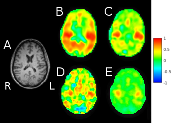
In Vivo: Results show this methodology removes false positive connectivity in white/gray matter when mapping major resting state networks at both low/high frequency (Fig.5). This methodology shows significant improvements to inherently low signal6, high frequency correlation maps, allowing for consistent observation of auditory networks across multiple subjects. Additionally, wSCA is shown to be comparable and complementary to regression techniques in a concurrent study7.
Discussion and Conclusion
As shown, wSCA allows for computationally efficient high pass filtering, noise reduction, and confound suppression. We have shown the benefits of this methodology that, while mathematically intricate, are analytically and numerically quantifiable. While traditional despiking methods8-10 provide stronger spike suppression, they require the ability to reliably identify isolated signal events and do not account for more complex confound waveforms. Therefore, wSCA is particularly advantageous for mapping high frequency connectivity where artifact characteristics are less well established. Additionally, this approach is well suited to single subject and real time applications, as it is computationally efficient and does not require a-priori knowledge of signal characteristics. Current efforts are focused on extending this methodology to probe the dynamics of resting state connectivity, which are of interest for characterizing neurological and psychiatric diseases.
Acknowledgements
We would like to thank Balasubramanian Santhanam for his guidance on filter design. Special thanks to Arvind Caprihan and Yin Yang for their advice on sliding window correlation. Diana South and Catherine Smith provided expert assistance with scanner operations. Our sincere gratitude to those team members whose work we continually build upon, including: James Thrasher, Elena Ackley, Kunxiu Gao, Radu Muthiac, and Vineeth Yeruva.References
1. Biswal, B., Yetkin, F. Z., Haughton, V. M., and Hyde, J. S. Functional connectivity in the motor cortex of resting human brain using echo-planar MRI. Magn. Reson. Med. 1995;34:537-541.
2. Greicius, M. D., Krasnow, B., Reiss, A. L., and Menon, V. Functional connectivity in the resting brain: A network analysis of the default mode hypothesis. PNAS, 2002;100(10):253-258.
3. Posse, S., Ackley, E., Mutihac, R., et al. High-speed real-time fMRI using multi-slab echo-volumar imaging. Front. Hum. Neurosci. 2013;7:479.
4. Posse, S., Ackley, E., Mutihac, R., et al. Enhancement of temporal resolution and BOLD sensitivity in real-time fMRI using multi-slab echo-volumar imaging. NeuroImage, 2012;61:115-130.
5. Gao, K. and Posse, S. TurboFire: Real-Time fMRI with Automated Spatial Normalization and Talairach Daemon Database, NeuroImage, 2003;19(2):838.
6. Chen JE and Glover GH. BOLD fractional contribution to resting-state functional connectivity above 0.1 Hz. Neuroimage, 2015;107:207-18.
7. Vakamudi, K., Damaraju, E., and Posse, S., . Enhanced Confound Tolerance of Resting fMRI: Combining Regression and Sliding-Window Meta-Statistic. OHBM 2016.
8. RW Cox. AFNI: Software for analysis and visualization of functional magnetic resonance neuroimages. Computers and Biomedical Research, 1996; 29:162-173.
9. RW Cox and JS Hyde. Software tools for analysis and visualization of FMRI Data. NMR in Biomedicine, 1997;10:171-178.
10. S Gold, B Christian, S Arndt, G Zeien, T Cizadlo, DL Johnson, M Flaum, and NC Andreasen. Functional MRI statistical software packages: a comparative analysis. Human Brain Mapping, 1998;6:73-84.
Figures
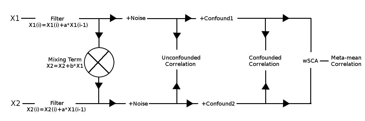
Flow chart showing the data simulation and analysis pipeline. Random signals are initially generated (X1 and X2) with a mean of 0 and variance of 1. A simple autoregressive filter is applied if frequency dependence is of interest, and a mixing term is introduced to induce a correlation in the signals. Gaussian noise is added to both signals and the correlation is calculated for reference. Confounds of interest are introduced, and the correlation is once more calculated. Finally, the wSCA methodology is implemented to measure the 'meta-mean' correlation.