Introduction

In functional magnetic resonance imaging (fMRI), the measured signal is assumed to be a linear convolution of neuronal response and the hemodynamic response function (HRF)¹. The variability of HRF has been widely recognized² and various models of the evoked HRFs have been investigated^3,4. However, current models involve simplified estimations of HRF and focus on limited frequency ranges, therefore, they are not suitable to analyze fMRI data with a higher frequency band. In this study, we proposed a new HRF estimation method, where we set a larger range of HRF parameters to cover wider frequency range and explicitly include a regularization term to penalize the curvature of the HRF and guarantee a smoothed estimated function. The new method is validated with both simulated data and real event-related fMRI data.

Methods

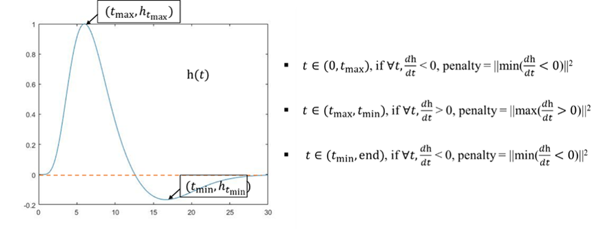
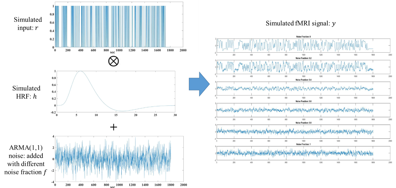
Model: We parameterized the estimated HRF model as a combination of the canonical HRF and its first order temporal derivative:$$$h(t) = (t^{a_2}-a_3t^{a_4})+a_5(e^{-t}(a_2t^{(a_2-1)}-a_3a_4t^{(a_4-1)})-e^{-t}(t^{a_2}-a_3t^{a_4}))$$$, where $$$a_2,a_3,a_4,a_5$$$ and are the unknowns of $$$h$$$. Let $$$y$$$ be a vector representing the time course from one voxel and $$$r$$$ represents n functions used to model the fMRI task design, the optimization problem here is: $$$||y-r*h||^2+\lambda\times$$$penalty, where $$$*$$$ denotes convolution. In Fig. 1, we explained the penalty term we used in detail. This non-smooth optimization problem was solved with the Broyden-Fletcher-Goldfarb-Shanno (BFGS) algorithm and inexact line search method⁵. A wide range of possible HRFs were generated and then clustered into 100 clusters based on their shape profiles using k-means clustering. The corresponding parameters of each cluster center were used as 100 starting points of BFGS algorithm. Simulation: A sequence of inputs with same amplitude and a duration of 3 seconds were generated as hypothetical task events (Fig. 2, left top). These events were then convolved with a hypothetical HRF (Fig. 2, left middle). The resultant signal was downsampled to mimic a TR of 0.765 seconds (same as our real fMRI data). Autoregressive moving average model (ARMA (1, 1))6 noise (Fig. 2, left bottom) was then added to the downsampled signal with different noise fractions to obtain simulated fMRI signals at different noise levels (Fig. 2, right). Imaging: Functional MRI was performed on 5 healthy subjects (age: 18 to 22) on a 3T Trio Tim Siemens MRI scanner (32-channel head coil, multiband accelerate factor = 8, TR/TE/flip angle = 765ms/30ms/44deg, 80 slices in oblique coronal orientation perpendicular to long axis of hippocampus, resolution 1.65mm x 1.65mm x 2mm, BW = 1724 Hz/pixel, echo spacing = 0.72 ms and 2380 time frames). An event-related repetition suppression spatial memory task was performed, involving viewing pairs of visual objects presented for the first time, repetitions of the same objects, or lures that were visually similar to the first-time objects. A control task (pixelated background of the math task) occurred occasionally requiring subjects to perform simple addition. Each task was on for three seconds and the blank between tasks was one second. Activations in the hippocampus were located and HRFs were estimated for every voxel in each hippocampal subregions.

Results

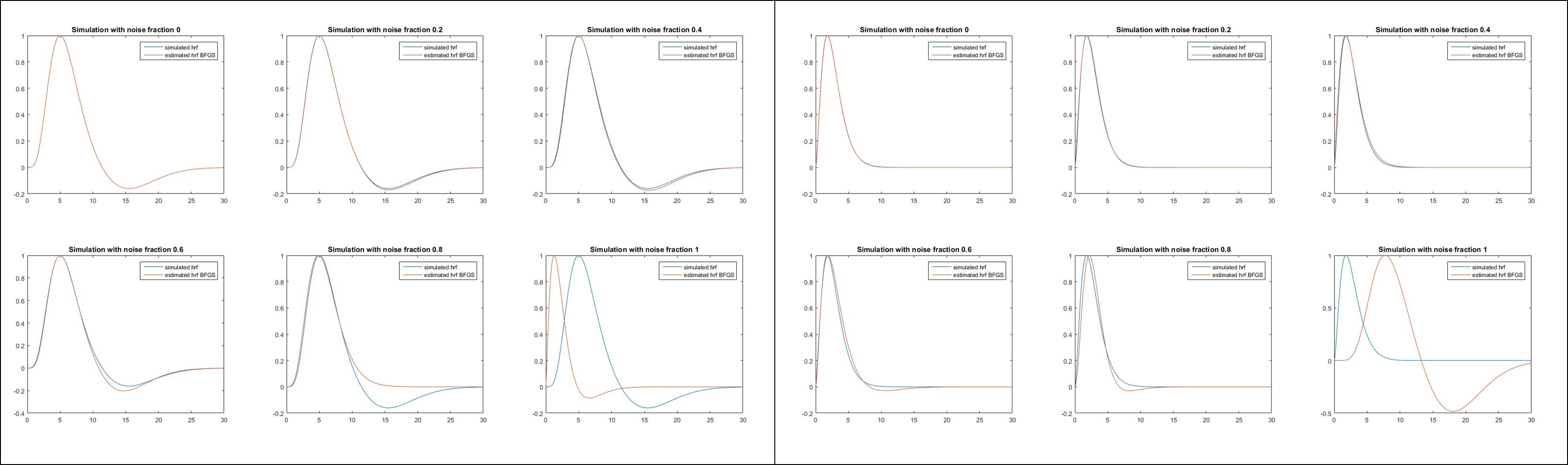
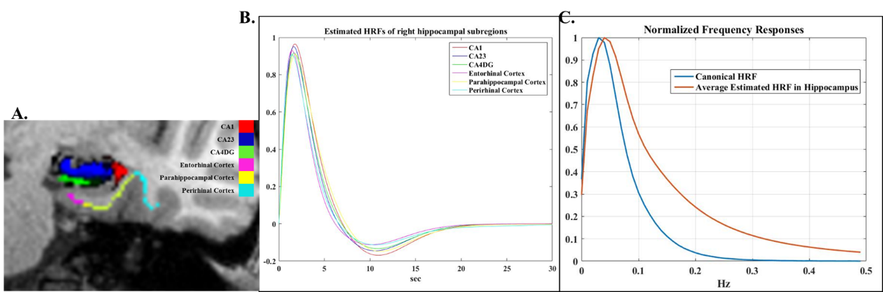
Fig. 3 shows two simulated HRFs (blue), at low and high frequency band, respectively, and the estimated results (red) obtained from simulated signals with different noise levels. For simulations with noise fraction 80%, the maximum difference between estimated HRF and simulated HRF is 16.28%. A full run of possible HRFs are tested and the highest estimation difference is less than 20% (when 80%). In real fMRI spatial memory dataset, bilateral activations in the hippocampus are observed for every contrast of memory v/s control. Hippocampal subfields and the estimated HRFs of each subregions, averaging over all active voxels are shown in Fig. 5 (A) and (B), respectively. Frequency responses of the canonical HRF and the obtained estimated HRF are shown in Fig. 5(C).

Discussion

Simulation results indicate that the proposed method is able to accurately recover HRFs with wider frequency band (Fig. 4). In validation with real event-related fMRI data, estimated HRF in hippocampal subregions shows a much shorter time to peak (Fig. 5(B)) and a higher frequency band (Fig. 5(C)), as compared to the canonical HRF. This may due to the subjects recruited in this study are relatively younger.

Conclusion

A new method of estimating HRF is proposed and solved with optimization techniques. Results from simulated data demonstrate the reliability of this method. Results from an event-related fMRI dataset further demonstrate the ability of the proposed method in capturing the variation of HRFs across different brain regions and subject populations.

Acknowledgements

The study was supported partially by the National Institutes of Health (grant number 1R01EB014284) and by National Institute of General Medical Sciences (grant number P20GM109025).