5323
Accounting for serial correlation in GLM residuals during resting state fMRI nuisance regression1Sir Peter Mansfield Imaging Centre, School of Medicine, University of Nottingham, Nottingham, United Kingdom, 2Division of Clinical Neurosciences, School of Medicine, University of Nottingham, United Kingdom, 3CUBRIC, School of Physics and Astronomy, Cardiff University, United Kingdom
Synopsis
In resting-state fMRI nuisance regression, a General Linear Model (GLM) is employed to fit and remove the variance associated with a noise model. Without "ground-truth" knowledge, the noise models must be tested and improved to obtain accurately cleaned datasets without "throwing the baby out with the bath-water." Valid statistical inference on a GLM fit requires normally-distributed residuals, which is not the case when intrinsic brain fluctuations are present. We demonstrate that existing pre-whitening tools can be appropriately applied to account for serial autocorrelation in resting-state fluctuations during nuisance regression, allowing statistical differentiation of true and simulated noise models.
Purpose
In typical resting-state experiments, we model numerous noise sources, and any signal not accounted for by our noise model becomes the de facto representation of intrinsic brain activity. This nuisance regression is typically achieved using a General Linear Model (GLM). However, to have valid statistical inference on the model fit parameters, normally-distributed GLM residuals are required. This is not the case when intrinsic neural fluctuations are present. Here we test whether modelling serial correlation in the residuals (e.g., pre-whitening) improves our interpretation of noise models in resting-state fMRI.Methods
fMRI acquisition
Twelve healthy subjects (32±6 years, 5 female) were scanned using a 3T GE HDx scanner (Milwaukee, WI, USA) equipped with an 8-channel receive head coil. A 5.5-minute eyes-open resting-state scan was acquired1 using a BOLD-weighted gradient-echo echo-planar imaging sequence (TR/TE=2000/35ms; FOV=22.4cm, 35 slices, resolution=3.5x2.5x4.0mm3, 165 volume acquisitions). The data were volume registered, motion corrected, time-shifted to a common temporal origin, and brain extracted (AFNI2, http://afni.nimh.nih.gov/afni) and 5 initial volumes were removed.
True noise model
Cardiac pulsations were monitored via finger plethysmograph and beat-to-beat heart rate was calculated. Expired CO2 content was monitored via nasal cannula (AEI technologies, PA, USA) and end-tidal values (PETCO2) extracted. Heart rate and PETCO2 data were smoothed using a CRF and HRF function, respectively3. Combined with the six head motion regressors derived during motion correction, these comprised the “true noise model.”
Simulated noise models
To form our null hypothesis, we simulated two additional noise models unrelated to the fMRI data: the noise model from a different subject, and a noise model consisting of phase-randomised versions of the true nuisance regressors (maintaining the inherent frequency content4).
Model fitting
The variance associated with the true or simulated noise models was removed from the data of each subject using 3dDeconvolve and 3dREMLfit2. 3dDeconvolve is a standard GLM programme with no pre-whitening, whereas 3dREMLfit accounts for serial autocorrelation in the GLM residuals, modelling them as an ARMA(1,1) process using Restricted Maximum Likelihood (REML). Additional parameters were included to detrend the data, removing baseline values and linear/quadratic trends.
To ascertain whether they were appropriately whitened, the 3dREMLfit residuals (original data minus the noise model fit and the modelled serial correlations) were assessed for remaining autocorrelation using the Durbin-Watson statistic. Note these residuals are not the "cleaned time-series": these can be calculated by subtracting the noise model fit from the original data. The R2 of the noise model (not including detrending terms) was extracted for each voxel, and an uncorrected threshold of p<0.05 was used to identify voxels where the fit was significant.
Results and Discussion
The ARMA(1,1) model used in 3dREMLfit appeared satisfactory for modeling the serial autocorrelation in the fMRI intrinsic brain fluctuations. No voxels demonstrated evidence of positive autocorrelation in the residuals, and only 4.5±0.1% of brain voxels showed evidence of remaining negative autocorrelation (mean±stdev across subjects).
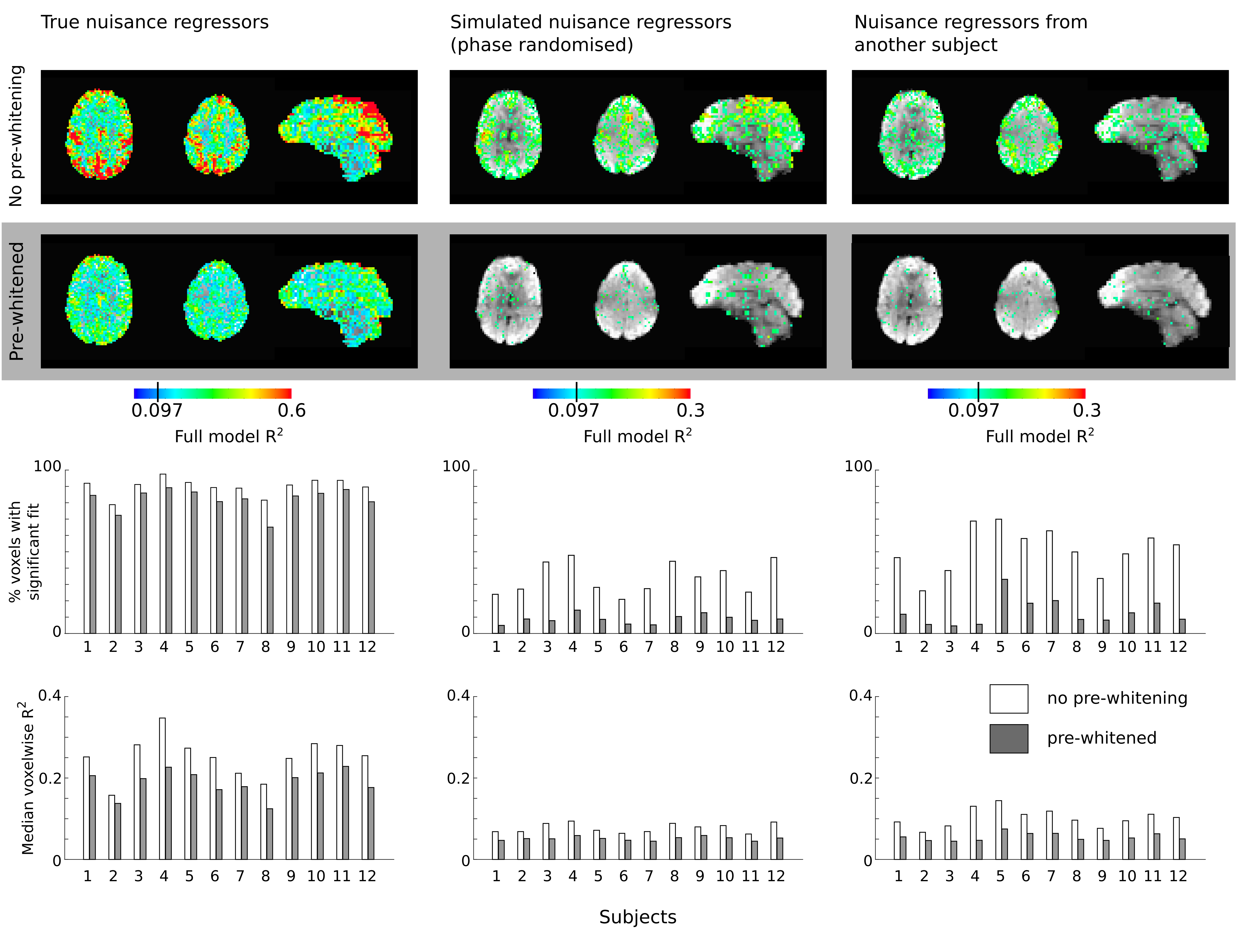
The fitting results are summarised in Figure 1. The median voxelwise R2, which approximates the percentage variance removed by the noise model, was reduced by 24% (true noise model), 45% (phase-randomised model), and 33% (incorrect subject model) following pre-whitening. This is consistent with the hypothesis that pre-whitening will impact true relationships less than it will spurious relationships between the noise model and the data, however it cannot be easily interpreted without "ground-truth" knowledge of the true contributions of different noise sources.
Similarly, pre-whitening reduced the number of voxels where the model fit was significant in all cases (paired t-tests, p<0.05, Bonferroni corrected). However, the size of this effect was dependent on whether the noise model consisted of true or unrelated, simulated regressors. When the true noise model was assessed, the percentage of brain voxels where the model fit was significant was reduced by only 9% due to pre-whitening, whereas it was reduced by 76% and 74% for the phase-randomised and incorrect subject noise models, respectively. This number of "false positives" was reduced to 13% (phase-randomised model) and 9% (incorrect subject model) of brain voxels, which exceeds an expected 5% false positive rate. This may be due to temporal correlation between the simulated and true nuisance regressors.
Conclusions
The incorporation of pre-whitening, or modeling serial correlation in the GLM residuals, to the nuisance regression pipeline allows valid statistical inference of model fit parameters, and reduces the presence of "false positives" when fitting a simulated, unrelated noise model to the data. Existing pre-whitening tools in standard software packages appear sufficient and can be easily applied. Ensuring correct usage of the GLM in denoising resting-state fMRI will allow accurate future optimisation of noise models and emerging nuisance regressors.Acknowledgements
MB is supported by the Anne McLaren Fellowship; KM is funded by the Wellcome Trust [WT200804].References
1. Bright, M. G., & Murphy, K. (2013). Reliable quantification of BOLD fMRI cerebrovascular reactivity despite poor breath-hold performance. NeuroImage, 83C, 559–568.
2. Cox, R. W. (1996). AFNI: software for analysis and visualization of functional magnetic resonance neuroimages. Computers and Biomedical Research, an International Journal, 29(3), 162–173.
3. Chang, C., Cunningham, J. P., & Glover, G. H. (2009). Influence of heart rate on the BOLD signal: The cardiac response function. NeuroImage, 44(3), 857–869.
4.
Bright, M. G.,
& Murphy, K. (2015). Is fMRI “noise” really noise? Resting state nuisance
regressors remove variance with network structure. NeuroImage, 114(C),
158–169.
Figures