Purpose

Chemical Exchange Saturation Transfer (CEST) MRI is sensitive to low-concentration metabolites such as creatine¹, glucose^2,3 and changes in microenvironment properties such as temperature⁴ and pH^5,6, promising in a host of in vivo applications such as imaging of ischemic stroke^7,8 and tumor^9,10. In vivo CEST quantification remains challenging due to concomitant effects such as RF spillover, semisolid macromolecular magnetization transfer (MT) and nuclear overhauser effects (NOE). Recently, least-squares fitting of Z-spectrum at low irradiation powers using a multi-pool Lorentzian model have been employed to resolve contributions from APT, spillover, MT, NOE, etc^11-14. However, the fitting reliability depends strongly on image signal-to-noise ratio (SNR), initial values and boundary values, which can lead to inaccurate fitting results, if not properly selected. In this study, we proposed an Image Downsampling Expedited Adaptive Least-squares (IDEAL) fitting algorithm that quantifies CEST images based on initial values from multi-Lorentzian fitting of iteratively less downsampled images.

Methods

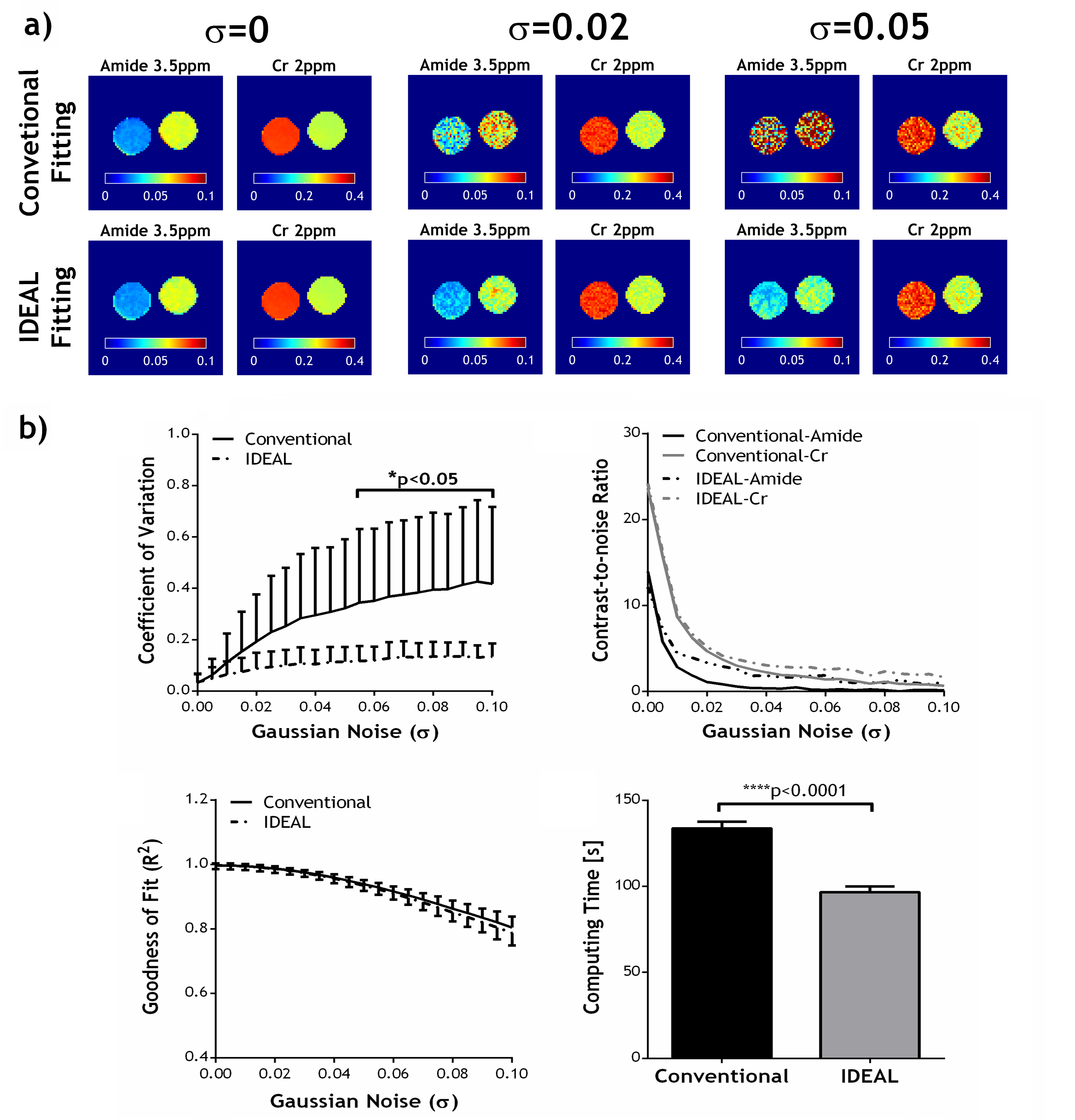
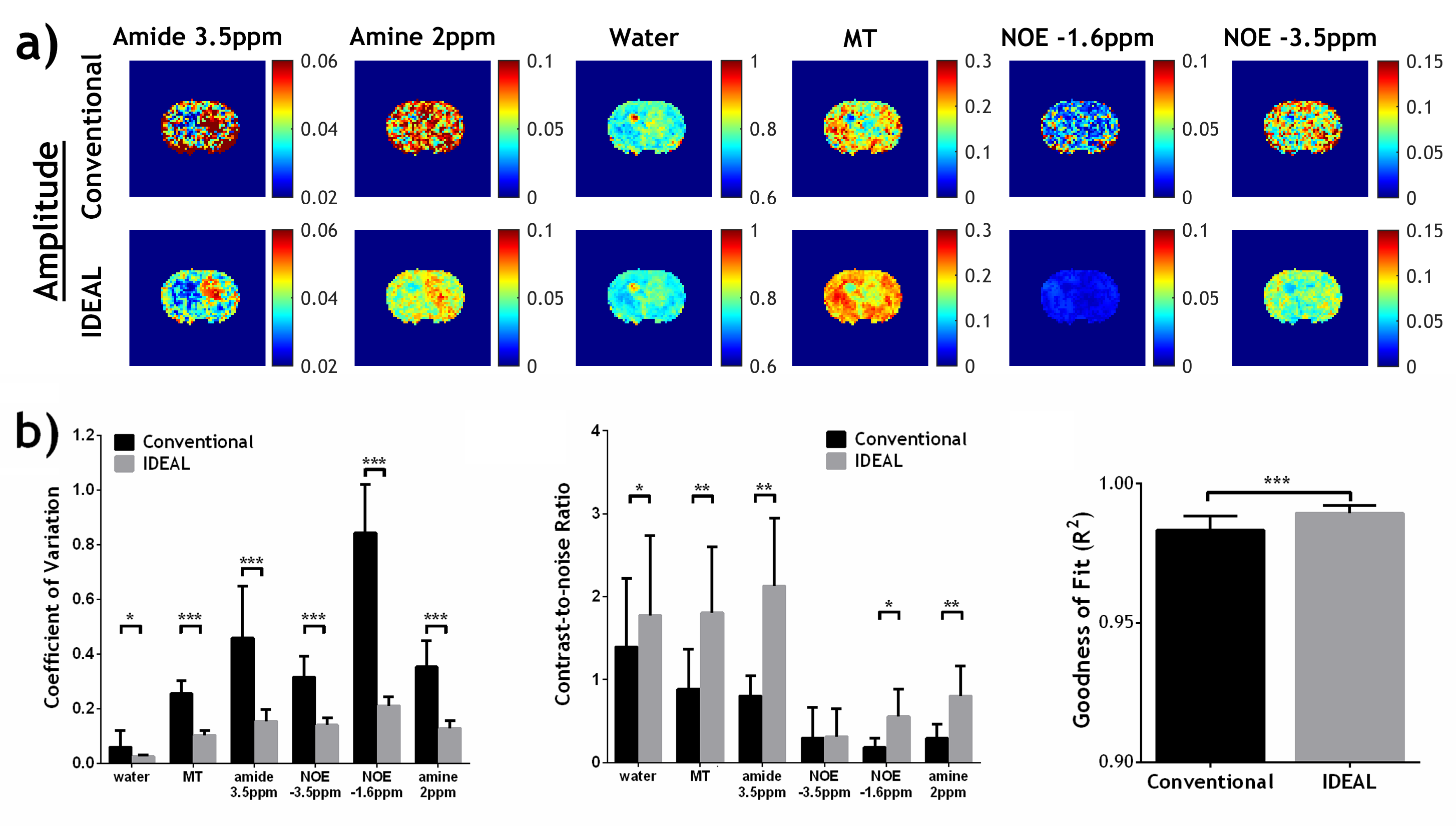
For phantom study, we used mixed mixed creatine (Cr) and nicotinamide (amide) in CuSO4-doped (1.5 mM) phosphate-buffered saline. Non-infiltrating D74 gliomas were developed in Fischer rats (N=8) as previously described¹⁵. The animals were imaged 11-13 days after tumor implantation. All MRI scans were performed on a 4.7T Bruker scanner. In vivo Z-spectrum was acquired from -6ppm to 6ppm with intervals of 0.25ppm and B₁=0.75µT, TR/TS/TE=10s/5s/15ms, 2 averages, scan time=8min20s. Conventional voxel-wise fitting of the Z-spectrum using a six-pool Lorentzian model of water (0 ppm), MT (-2 ppm), amide (3.5 ppm), amine (2 ppm) and NOE effects at -3.5 ppm and -1.6ppm was performed with loosely constrained bounds between 10% and 10 times of the initial values for amplitude and linewidth, and ±20% of the corresponding linewidth for offset of each proton pool. The proposed IDEAL fitting method uses globally averaged Z-spectrum for initial fitting with the same relaxed boundary constraints, which are more reliable given the high SNR. The initial fitting results are then used as initial values for subsequent voxel-wise fitting of substantially downsampled CEST images with tightly constrained bounds of ±10% these initial values for amplitude and linewidth, and ±5% of the corresponding linewidth for frequency offset. The resolution of downsampled images is increased iteratively and fitted with the fitting results from the previous downsampled images as renewed initial values until the original image resolution is reached. The quality of fitting was evaluated by coefficient of variation (COV, i.e., standard deviation/mean), contrast-to-noise ratio (CNR) and goodness of fit (R²) maps. To evaluate the performance of the fitting methods under noise, different levels of Gaussian noise with σ ranging from 0.005 to 0.1, were added to the original phantom data.

Results and Discussion

No significant difference was found in the fitted amplitudes of amide and Cr peaks between conventional fitting and IDEAL in the absence of simulated noise (Fig1a, σ=0), while strong variation in fitted maps was induced by superimposed noise (Fig1a, σ=0.02 and 0.05). Fig. 1b shows that the IDEAL fitting in phantom data with superimposed noise provided smaller COV and higher CNR at a faster fitting speed compared to conventional fitting. We further applied the IDEAL fitting to quantify the contributions from APT, amine, NOE and MT effects in a rat model of glioma (Fig2a). Fig2b shows IDEAL fitting provides significantly smaller COV for all the fitted pools and more importantly, substantially higher CNR in five out of the six pools with higher R². For all the gliomas studied (N=8), both methods showed significantly increased APT, reduced MT and no change in NOE-3.5ppm in the tumor. Interestingly, the IDEAL fitting revealed pronounced negative contrasts in tumors in the fitted CEST maps at 2ppm and -1.6ppm which were not found using conventional method due to strong variation in its fitting results. These CEST contrasts may reflect changes in creatine level^1,19 and NOE effects²⁰, warranting further investigation of their potentials in tumor detection, grading and treatment. It is anticipated that the proposed IDEAL fitting can be generalized to quantify MRI dataset where SNR is suboptimal.

Acknowledgements

No acknowledgement found.