Synopsis

Magnetic resonance fingerprinting (MRF) is a technique that enables simultaneous quantification of tissue parameters in a single scan. So far, MRF has been realized mostly for clinical 1.5 T and 3 T scanners, and a preclinical 7 T scanner. Application to a higher field scanner is limited and challenging because of the increased sensitivity to system hardware imperfections, such as B0 and B1 inhomogeneities and slice-profile imperfection. In this study, we assessed the feasibility of the MRF approach in a preclinical, wide-bore 14.1 T system.

Introduction

Methods

The MRF was implemented on the 14.1 T MRI system (Bruker AVANCE III 600 MHz Wide Bore NMR/MRI Spectrometer, Bruker Inc) with a 40 mm inner diameter gradient insert with up to 1.47 T/m gradient strengths (Bruker Micro2.5 gradient system) and a 30 mm inner diameter quadrature coil (MicWB40, Bruker Inc.). The samples were CuSO₄–doped water phantoms with varied concentrations and a tomato fruit.

The MRF acquisition was developed from a fast imaging with steady-state free precession (FISP) ^2,3. The MRF acquisition was initiated with an adiabatic inversion pulse (4.84 ms duration), which was followed by 300 successive FISP acquisition periods with varying flip angel (FA) and repetition time (TR). Echo time (TE) was held constant (4 ms). FA and TR were determined by pseudo-randomly according to the method proposed by Gao et al.³. FA was varied sinusoidally (5 to 90^o) and TR was varied using a Perlin noise pattern (20 to 30 ms). For the acquisition of the MRF signal evolutions, the same line of k space for each of 300 sequential images during each MRF scan repetition period (whole TR) was measured.

The MRF dictionary was created using a home-written extended phase graph simulator, which was implemented in a C/C++ programming environment. The MRF dictionary consisted of 137280 profiles generated from 24 T₁ values (20-600 ms), 44 T₂ values (20-600 ms: increment, 20 ms) and 25 B₁ values for the CuSO₄-doped water measurement and 218736 for the tomato measurement. Unrealistic profiles with T₁<T₂ were excluded. The dictionary was matched to the acquired MRF signal evolution profile using vector-based inner product comparisons.

Results and discussion

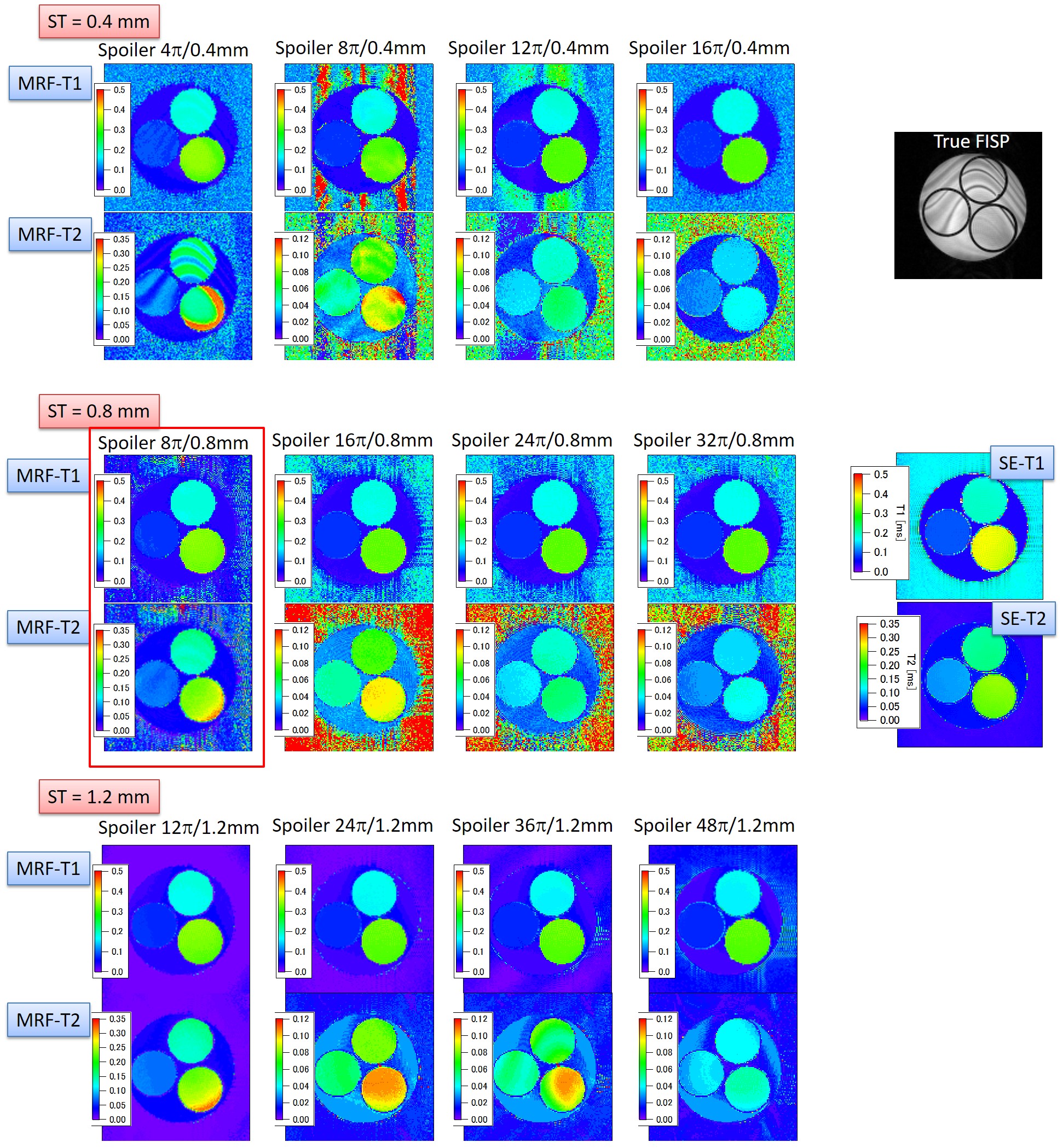
The MRF-FISP results varied, depending on the slice thickness (ST) and spoiler gradient moment (Fig. 1). Although the MRF-T₁ estimates were not significantly different, the MRF-T₂ estimates were different from each other. The MRF-T₂ map suffered from the banding artifacts for ST = 0.4 mm and the smaller moment. These artifacts, which also appeared in the trueFISP image, were caused by the field inhomogeneity. In general, the banding artifacts tend to be remarkable in the high-field-strength and wide field-of-view scanners. Under the current experimental setup, the field homogeneity needed to be no lower than ~0.03 ppm over a 30 mm diameter spherical volume to avoid banding artifacts. For the system we used, this could not be satisfied even with the automated, localized third-order shimming.

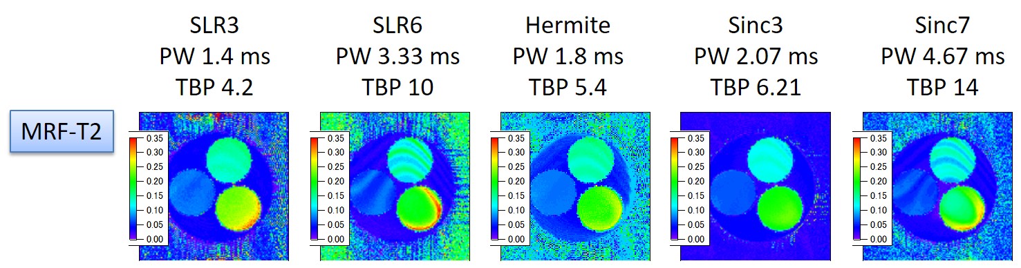
As shown in Fig. 1, the banding artifacts could be alleviated by increasing the spoiler gradient moment, but it also caused a decrease in the T₂ value possibly because of the diffusion weighting. Therefore, there is a tradeoff between the banding-artifact alleviation and T₂ accuracy. For ST = 1.2 mm, the MRF-T₂ map showed another artifacts, possibly because of the large B₀ inhomogeneity in a voxel. The MRF-T₂ estimate also depended on the slice profile (Fig. 2). The banding artifacts less appeared for the profiles with the smaller time-bandwidth products (TBPs), possibly because spins in one voxel were less coherent and they were effectively dephased.

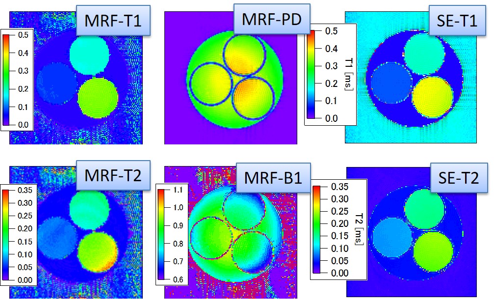
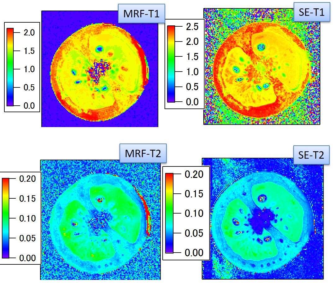
Figure 3 shows the MRF results obtained under an optimum condition (ST = 0.8 mm; moment = 8π/0.8 mm; SLR3 pulse). Figure 4 shows the MRF-T₁ and T₂ maps of a tomato fruit, which was obtained under the above optimum condition. There were less banding artifacts in the images and the MRF-T₂ estimates corresponded to the spin-echo based estimates. The MRF-T₁ estimates were smaller than the inversion-recovery based estimates, possibly because the whole TR was short and T₁ saturation was not fully recovered. This could be corrected by selecting a longer whole TR.

Conclusion

Acknowledgements

References

1. Ma D, et al. Magnetic resonance fingerprinting, Nature 2013;495:187-193.

2. Gao Y, et al. Preclinical MR fingerprinting (MRF) at 7 T: effective quantitative imaging for rodent disease models, NMR Biomed. 2015;28:384-394.

3. Jiang Y, et al. MR Fingerprinting Using Fast Imaging with Steady State Precession (FISP) with Spiral Readout, Magn. Reson. Med. 2015;74(6):1621-31.