5200
Comparison of MRI techniques for hepatic fat and iron quantification in the UK Biobank study1Perspectum Diagnostics, Oxford, United Kingdom
Synopsis
We compared standard Dixon and T2* relaxometry with “IDEAL” for measuring liver proton density fat fraction (PDFF) and T2*, surrogate metrics for steatosis and iron burden respectively. Results in 118 UK Biobank study participants showed very good correlation between the two methods. Dixon PDFFs were consistently lower than IDEAL PDFFs, explained by the 20° flip angle used for Dixon, introducing a T1 bias and deviation from true PDFF values. Results also showed improved image quality for IDEAL, highlighting the strength of this technique to serve as a reliable and simultaneous biomarker of liver fat and iron overload.
Purpose
Steatosis and iron overload are two of the key features of chronic liver disease1. Quantitative MRI can provide surrogate metrics for these features and can contribute to the prediction of clinical outcomes2. In this study we compared different imaging techniques (the standard Dixon3 and T2* relaxometry methods versus the comprehensive “IDEAL” approach4-11), to measure proton density fat fraction (PDFF), and T2* for iron quantification in the liver. We performed measurements using both techniques in a subset of participants (>500) enrolled in the UK Biobank (UKB) study12. Our goals were to compare metrics and image quality between the two techniques. We also computed a mapping between the two measures that can be applied across all UKB study participants (>100,000), to provide population based biomarkers for use in prospective studies of liver disease.Methods
Single slice abdominal images from >500 participants were acquired at the dedicated Biobank Imaging Centre at Cheadle (UK), using Siemens 1.5T MAGNETOM Aera, with two different imaging protocols as shown in Table 1.
At time of writing, 120 cases have been processed. Protocol1 data were used to calculate PDFF maps using the 3-point Dixon method4 and T2* maps using a standard decay-curve fitting method. Using Protocol2 data, algorithms based on the IDEAL4-11 approach were used to calculate PDFF and T2* maps. The IDEAL implementation included corrections to address T2* decay6, the multi-spectral fat signal7, noise bias8, water/fat swaps9, and phase errors10.
Image quality was assessed visually, making note of the number of fat/water swaps and cases where physiological noise or motion artefacts were more noticeable in Protocol1 compared with Protocol2 maps. For image quantification of each PDFF and T2* map, 3 circular regions of interest (ROIs) of 15 mm diameter were manually placed (by CH), avoiding vessels and image artefacts. Mean and Coefficient of Variation (CV) were calculated from the ROI pixels.
Calculation of quantitative maps and analyses were all performed using algorithms implemented in LiverMultiScan2 post-processing software. PDFF calculation using the IDEAL implementation was validated using publicly available phantom data11.
Results
Two examples of PDFF and corresponding T2* maps calculated using the different protocols are shown in Figure 1. Of 120 datasets analysed, 21 showed noticeably higher levels of noise in Protocol1 (Dixon and standard T2* relaxometry) compared to Protocol2 (IDEAL) PDFF and T2* maps. Fat/water swaps were observed in 2 cases for Protocol1 and in one corresponding set for Protocol2, though such swaps are the subject of on-going work. These were excluded from further analyses.
ROI analyses showed very good correlation between the two protocols for PDFF (r=0.99) and for T2* (r=0.96). Regression slopes and intercepts were (1.21, 0.21) for PDFF, signifying that Protocol1 PDFF is consistently lower than Protocol2, especially at higher PDFF values (Figure 2, left), and (0.97, 1.01) for T2* (Figure 2, right). For T2*, there was no statistical evidence for difference between the two protocols.
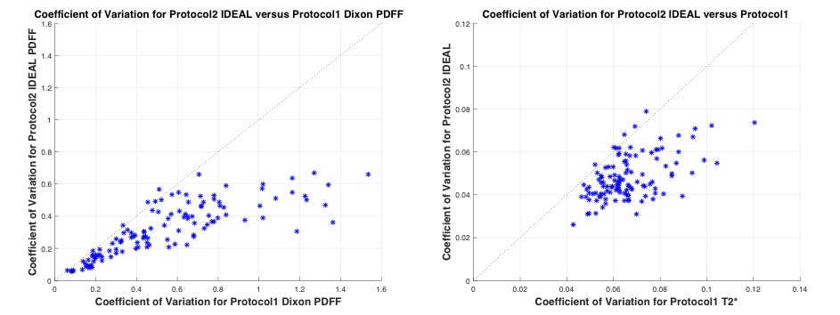
CV was used as a comparison of signal variation and hence noise levels between the two sets of measures. Figure 3 shows that for both PDFF (left) and T2* (right), CV is higher for Protocol1 than Protocol2 in the majority of cases (112/118).
Discussion
This study has demonstrated a very good correlation between two different measurements of PDFF and of T2*. Lower Protocol1 versus Protocol2 PDFF values (signified by regression slope of 1.21), can be explained by the 20° flip angle used for Protocol1, which introduced a T1 bias and hence deviation from true PDFF values8. However, given the strong correlation between the two PDFF measures, the linear regression can be used to correct Protocol1 PDFF values. Note that this mapping has currently been calculated using 118 participants, but will be recalculated for all data that were acquired using both techniques (>500 cases).
The qualitative and quantitative comparison between the techniques suggests that overall noise levels were lower for Protocol2 (IDEAL), which allowed for more rapid acquisition so that 6 averages could be acquired within a single breath-hold.
Conclusion
Our qualitative and quantitative comparison of two protocols measuring PDFF and T2* showed that Protocol2 (IDEAL) gave improved image quality, highlighting the strength of this technique to serve as a reliable and simultaneous biomarker of liver fat and iron overload.
Acknowledgements
We would like to acknowledge and thank the staff and participants of the UK Biobank StudyReferences
1. Banerjee R, Pavlides M, Tunnicliffe EM, et al. Multiparametric magnetic resonance for the non-invasive diagnosis of liver disease. J Hepatol. 2014; 60(1): 69–77.
2. Pavlides M. and Banerjee R. Multiparametric magnetic resonance imaging predicts clinical outcomes in patients with chronic liver disease. J Hepatol. 2016;64(2):308-315.
3. Glover GH. Multipoint Dixon technique for water and fat proton and susceptibility imaging. J Magn Reson Imaging. 1991;1(5):521-530.
4. Reeder SB, Wen Z, Yu H, et al. Multicoil Dixon chemical species separation with an iterative least-squares estimation method. Magn Reson Med. 2004;51(1):35-45.
5. Reeder SB, McKenzie C, and Pineda A. Water-fat separation with IDEAL gradient-echo imaging. J Magn Reson Imaging. 2007;25(3):644-652.
6. Yu H, McKenzie CA, Shimakawa A, et al. Multiecho reconstruction for simultaneous water-fat decomposition and T2* estimation. J Magn Reson Imaging. 2007;26(4):1153-1161.
7. Yu H, Shimakawa A, McKenzie CA, et al. Multiecho water-fat separation and simultaneous R2* estimation with multifrequency fat spectrum modeling. Magn Reson Med. 2008;60(5):1122-1134.
8. Liu CY, McKenzie CA, Yu H, et al. Fat quantification with IDEAL gradient echo imaging: correction of bias from T(1) and noise. Magn Reson Med. 2007;58(2):354-364.
9. Yu H, Reeder SB, Shimakawa A, et al. Field map estimation with a region growing scheme for iterative 3-point water-fat decomposition. Magn Reson Med. 2005;54(4):1032–1039. ?
10. Yu H, Shimakawa A, Hines CD, et al. Combination of complex-based and magnitude-based multiecho water-fat separation for accurate quantification of fat-fraction. Magn Reson Med 2011;66(1):199–206.
11. Hernando D, Sharma SD, Aliyari Ghasabeh M, et al. Multisite, multivendor validation of the accuracy and reproducibility of proton-density fat-fraction quantification at 1.5T and 3T using a fat-water phantom. Magn Reson Med. 2016 Apr 15. doi: 10.1002/mrm.26228
12. UK Biobank. Available from: http://www.ukbiobank.ac.uk.
Figures
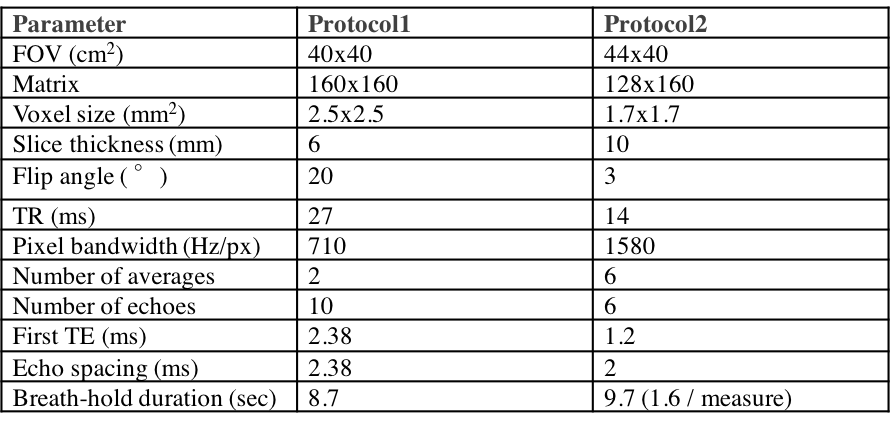
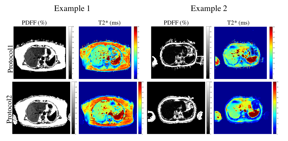
Figure 1 - Two examples of PDFF and T2* maps calculated using Protocol1 (Dixon and T2* decay-curve fitting) and Protocol 2 (IDEAL). Example 1 (left), Protocol1 PDFF = 12.69%, CV=0.13, T2*=23.02ms, CV=0.06, Protocol2 PDFF=16.71%, CV=0.07, T2*=23.94ms, CV=0.04. Example 2 (right) Protocol1 PDFF = 1.28%, CV=0.72, T2*=24.41ms, CV=0.07, Protocol2 PDFF=1.58%, CV=0.47, T2*=23.11ms, CV=0.03.
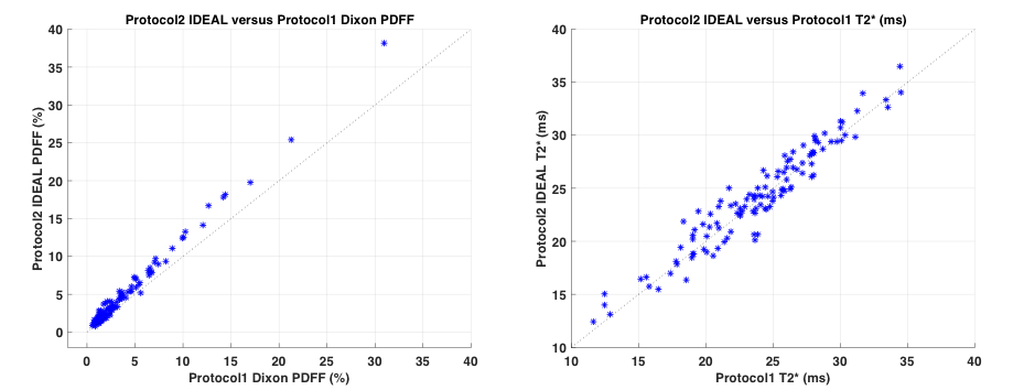
Figure 2 - PDFF (%) for Protocol2 (IDEAL) versus Protocol1 (Dixon) on left. T2* (ms) for Protocol2 (IDEAL) versus Protocol1 (decay-curve fitting) on right. Data shown for 118 cases analysed at time of writing.