5185
Classification of White and Brown Adipose Tissue using a Support Vector Machine1Physics and Astronomy, University of Georgia, Athens, GA, United States, 2Bio-Imaging Research Center, University of Georgia, Athens, GA, United States, 3Biochemistry and Molecular Biology, University of Georgia, Athens, GA, United States
Synopsis
Determining the volume and distribution of white adipose tissue (WAT) and brown adipose tissue (BAT) by magnetic resonance imaging (MRI) is clinically important. Previous WAT and BAT classification has relied on using fat fraction and proton relaxation time via fixed multi-peak spectroscopic models. However, the recently proposed Multi-Varying-Peak MR Spectroscopy (MVP-MRS) model allows for the selection of appropriate classification features for differentiation between WAT and BAT. Furthermore, these multi-peak features allow prediction of a ‘browning’ or ‘beigeing’ process of WAT by using a Support Vector Machine (SVM) learning algorithm.
Purpose
To differentiate white adipose tissue (WAT) from brown adipose tissue (BAT) post injection of CL3 in a mouse model via a Support Vector Machine (SVM) learning algorithm. The dynamic changes of WAT and BAT percentage over time can be used to predict a ‘browning’ or ‘beigeing’ process of WAT.Introduction and Methods
Determining the volume and distribution of BAT by in vivo imaging is clinically important.1 Previous methods assume a fixed multi-peak spectroscopic model for both WAT and BAT, and depend upon a fat fraction ratio and MR relaxation time to differentiate BAT from WAT.2 These fat fraction models have been shown to be inaccurate.3 MR spectra of BAT and WAT have shown a main peak (-(CH2)n-) at 1.3-ppm, accompanied by several other peaks located at 0.9, 2.1, 4.3, and 5.3 ppm corresponding to different structures of fatty acid (saturated vs. unsaturated). The Multi-Varying-Peak MR Spectroscopy (MVP-MRS) has been proposed4 which differs from previous methods by approximating individual fat resonance peaks independent of a fixed peak amplitude. The proposed MVP-MRS model is as follows
$$s(t)=(\rho_w + \sum_{n=1}^N \beta_n e^{j 2 \pi f_n t}) \cdot e^{j 2 \pi \phi t} \cdot e^{-R_{2,q}^* t}$$
where $$$\rho_w$$$ is the water proton density, $$$\ f_n$$$ and $$$\beta_n$$$ are the resonant frequency and varying proton density of the nth fat peak (N=5) relative to water, and $$$R_{2,q}^*$$$ is the transverse relaxation rate at each voxel q. Since the last two fat peaks (at 4.3 and 5.3 ppm) are close to the water peak (at 4.7 ppm), they are prone to noise corruption. Therefore, the first three fat peaks, water peak, and R2* were chosen as appropriate features for an SVM. SVMs are machine learning algorithms used to analyze data for classification.5 Training data is provided to the algorithm via n-number of features, with each n-dimensional data point labeled as one of two predetermined categories (e.g., WAT or BAT). The function of the algorithm is to determine an (n-1)-dimensional separating hyperplane that best separates the data in its feature space. The data points provided by the features proved to show a nonlinearly separable distribution of classification points, therefore a radial basis function kernel was required to create a transformed feature space to separate the data.
Data Acquisition
MR data was acquired from healthy C57/BL6 mice using a 7 T Varian Magnex small animal scanner. Mice were first scanned using a 2D multi-echo multi-slice sequence and a multi-echo 3D gradient-recalled echo (GRE) sequence before an i.p. injection with CL316,243 (1 mg/kg). The animals were then scanned at 45, 75, 135, and 175 minutes post injection.Results
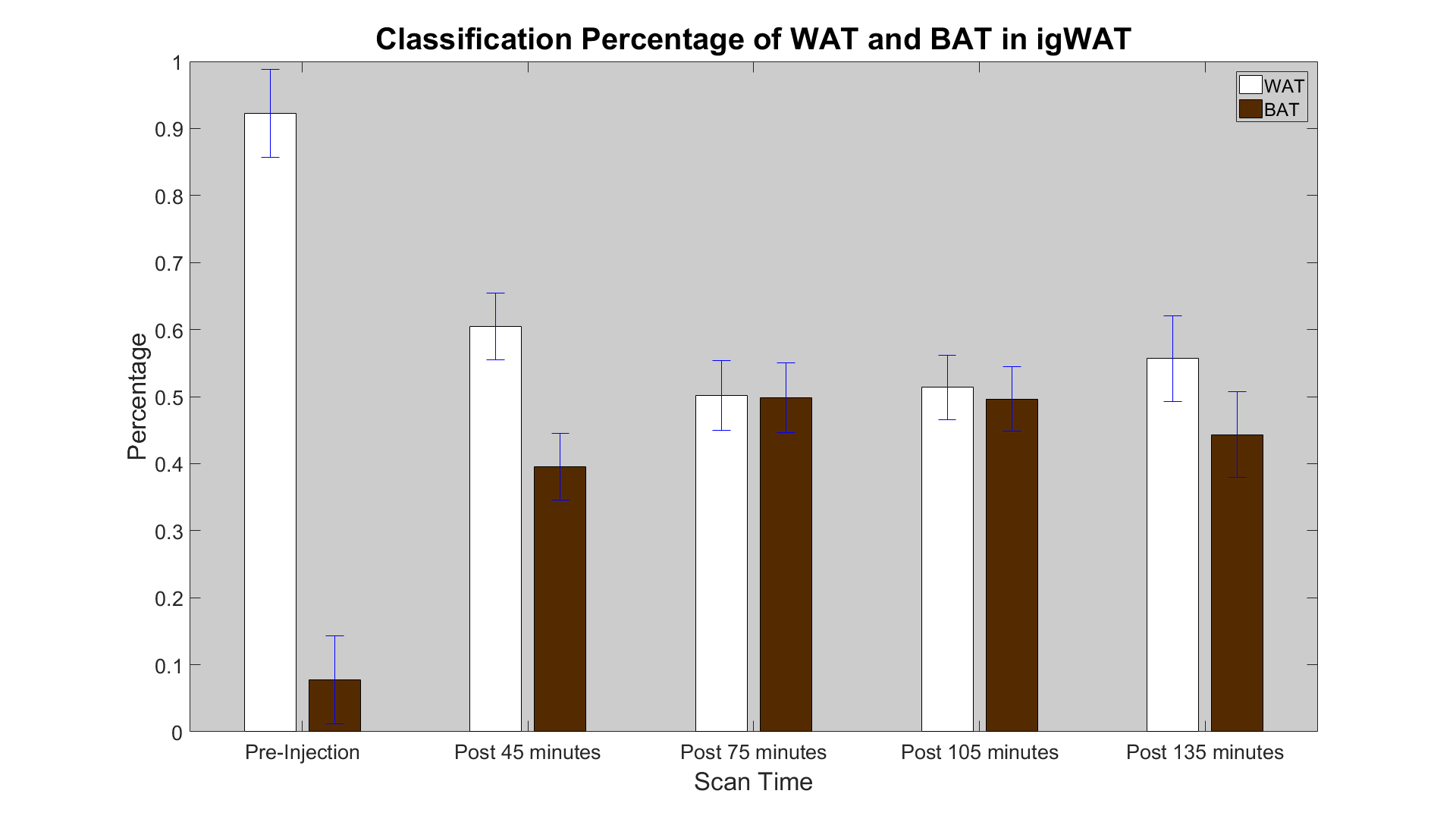
Water and fat data analysis was conducted with a modified MATLAB water-fat analysis toolbox (http://ismrm.org/workshops/FatWater12/data.htm). The training set data was selected from 36 voxels of pre-injection inguinal WAT (igWAT) and 123 voxels of intracapsular BAT. In order to observe if post-injection beigeing was occurring, test data (50 voxels each) was acquired from the same location as the igWAT training data but from the 4 post-injection time points. The train-test procedure was repeated 50 times, randomizing the training data each time. The SVM used a radial basis function with a fixed kernel size. Figure 1 shows the percentage of WAT and BAT in igWAT for pre- and post-injection time points. An increase of BAT percentage while a decrease of WAT percentage suggests a possible beiging process of the igWAT.
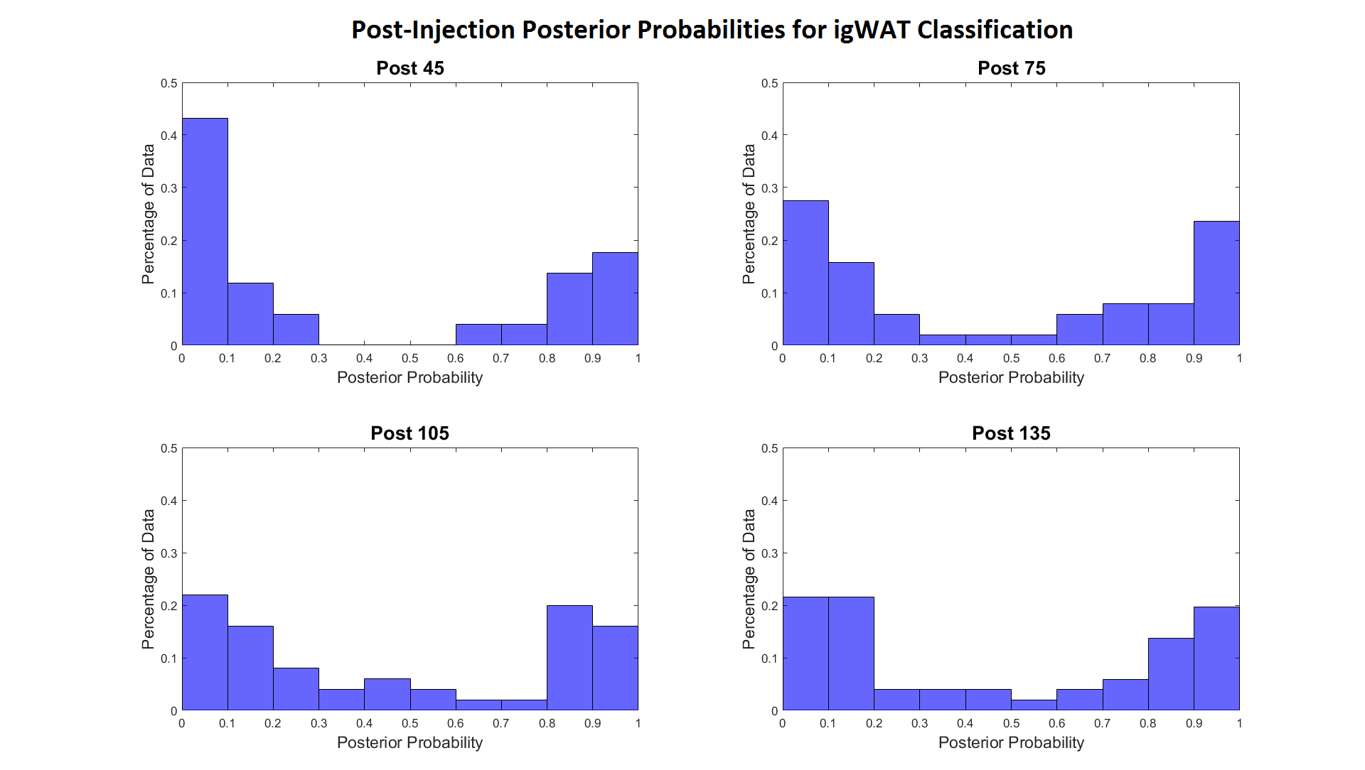
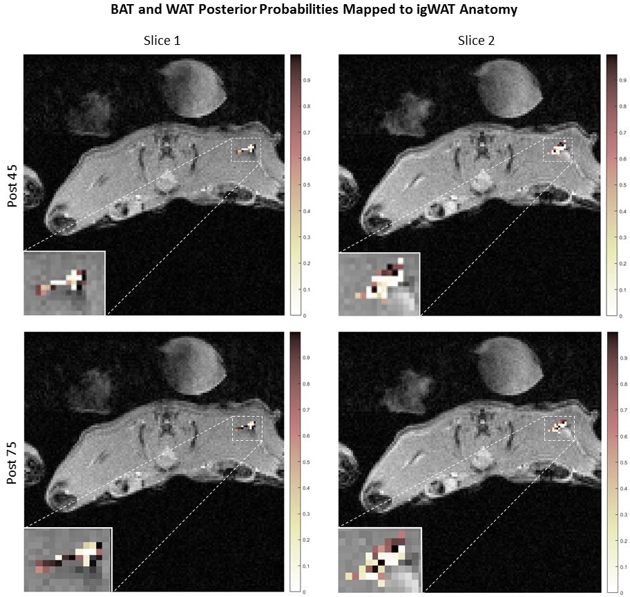
Figure 2 shows classification posterior probability values calculated for each time point. These probabilities are viewed as a confidence in classification of WAT and BAT. Again the data shows that as time increases, WAT and BAT were separated with high confidence (approaching 0 by the WAT group, and approaching 1 by the BAT group). The posterior probabilities were then mapped back onto the anatomy of the mouse to show a spatial distribution of the beiging process. Figure 3 illustrates a dynamic, inhomogeneous distribution of BAT among the igWAT area.
Discussion and Conclusion
The varying fat spectrum peaks introduced by the MVP-MRS model have shown to provide appropriate features for classification. The SVM classifications presented in this study show a clear division of WAT and BAT, which would be more difficult with the previous static peak models. The high confidence values provided by the posterior probabilities of each classification further support a possible beiging process of WAT in the region of interest with each time step. Another important aspect of the SVM is that inhomogeneous distributions of BAT and WAT can be determined and visualized using the posterior probability, which needs further confirmation by histology analysis.Acknowledgements
The authors wish to thank Drs. Diego Hernando (University of Wisconsin) and Houchun Hu (The Phoenix Children’s Hospital) for their helpful discussions.References
1. Cypess, A.M., et al., Identification and importance of brown adipose tissue in adult humans. N Engl J Med. 2009;360(15):1509-17.
2. Hamilton, G., et al., MR properties of brown and white adipose tissues. J Magn Reson Imaging. 2011; 34(2):468-73.
3. Zancanaro, C., et al., Magnetic resonance spectroscopy investigations of brown adipose tissue and isolated brown adipocytes. J Lipid Res. 1994;35(12):2191-9.
4. Simchick, G., J. Wu, G. Shi, H. Yin, and Q. Zhao, Characterization of Brown Adipose Tissue using Multi-Varying-Peak MR Spectroscopy (MVP-MRS), in Proceedings of the Annual Conference of International Society of Magnetic Resonance in Medicine. 2016: Singapore. P. 3280
5. Cortes C, Vapnik V. Support-vector networks. Machine Learning. 1995;20(3):273-297.
Figures