5177
Absolute B1- estimation without a homogeneous receive coil1Department of Medical Biophysics, The University of Western Ontario, London, ON, Canada, 2Centre for Functional and Metabolic Mapping, The University of Western Ontario, London, ON, Canada
Synopsis
Fitting the relative B1- maps derived from a B1+ shim acquisition to the Helmholtz equations allows for the calculation of absolute B1- maps. The sensitivity profiles can then be used to optimally combine coils in subsequent acquisitions. In addition, absolute B1- maps allow for the removal of the receive sensitivity from the combined images. This was validated in a GE-EPI sequence and found to produce images with lower phase standard deviation and increased temporal signal-to-noise ratios across the brain. Both of these differences were found to be statistically significant in a Student’s t-test.
Purpose
This study developed an absolute $$$B_1^-$$$ mapping procedure that does not rely on using a homogeneous receive coil, e.g. body coil, as $$$B_1^-$$$ heterogeneity increases at high field. The $$$B_1^-$$$ maps can be derived from the same acquisitions used to estimate $$$B_1^+$$$, therefore introducing no additional scan time. These can then be applied to subsequent images to allow for optimal coil combination (free of $$$B_1^-$$$ weighting).Methods
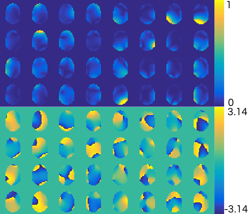
The individual coil images used for $$$B_1^+$$$ mapping1 are combined via singular value decomposition which also provides relative $$$B_1^-$$$ maps2. Estimation begins by masking of the relative $$$B_1^-$$$ maps in order to the determine the region for the fit. The masking is done through the ratio of the primary to secondary singular vector as a rough measurement of signal to noise ratio (SNR).
Assuming uniform electrical tissue properties, the $$$B_1^-$$$ should follow the Helmholtz equation. The solution to the Helmholtz equation that is finite at the origin is:
$$\triangledown^2B_1^-=-k^2B_1^-$$
$$B_1^-(r,\theta,\phi)=\sum_{l=0}^{l_{max}}\sum_{m=-l}^{l}c_{lm}j_l(kr)Y_l^m(\theta,\phi)$$
where $$$c_{lm}$$$ are the coefficients to be fitted, $$$Y_l^m$$$ are spherical harmonics and $$$j_l$$$ are spherical Bessel functions of the first order. The $$$B_1^-$$$ profiles are known to be spatially smooth allowing fitting to be completed up to limit order $$$l_{max}$$$.
The voxel-wise relative $$$B_1^-$$$ maps are scaled by the unknown complex scaling composed of the spatial $$$l_2$$$-norm and transmitter phase that is common to all coils. The $$$B_1^-$$$ maps are iteratively fit to the Helmholtz equation solution and a common scaling term. The fit uses a weighted least squares algorithm in order to find the appropriate coefficients. Then, the complex scaling is estimated as the weighted mean of the ratio between the fitted $$$B_1^-$$$ and the measured relative $$$B_1^-$$$. The scaling is then applied to the relative $$$B_1^-$$$ and the next iteration is completed. This is repeated until the fitted $$$B_1^-$$$ converges.
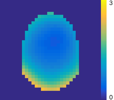
These fitted $$$B_1^-$$$ can then be applied to any scan during reconstruction. Because polynomial fits are inherently poor extrapolators, the fits are only used to interpolate within the convex hull of all fitted points. For points exterior to the convex hull the sensitivity of the closest point on the convex hull is used. The $$$B_1^-$$$ is applied to the complex image values (M) to generate magnetization (m) as follows2 ($$$^H$$$ is hermitian transpose):
$$S=\frac{\mathbf{({B_1^-})^H}}{\mathbf{({B_1^-})^H}\mathbf{{B_1^-}}}\mathbf{M}=\frac{\mathbf{({B_1^-})^H}}{\mathbf{({B_1^-})^H}\mathbf{{B_1^-}}}\left(\mathbf{{B_1^-}}m \right)=m$$
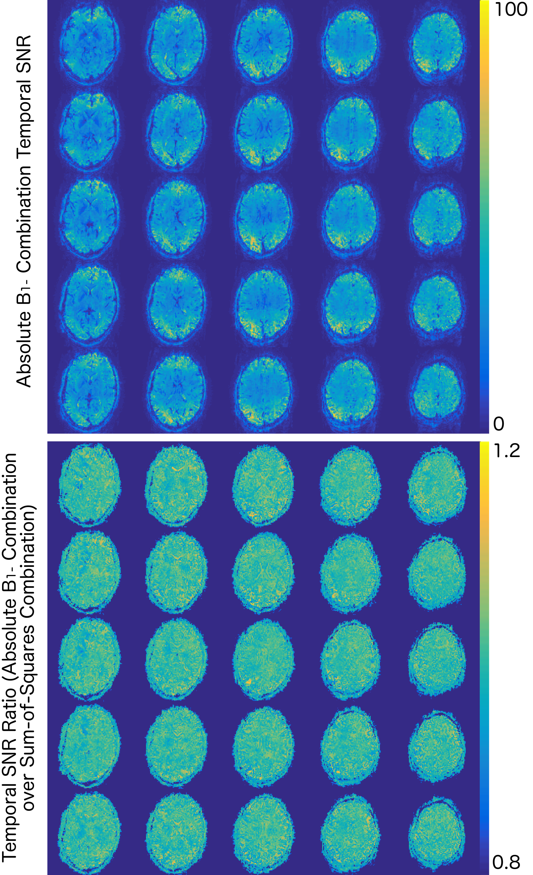
In order to validate this method, accelerated EPI scans were collected and reconstructed using standard system coil combination and receiver sensitivity weighted combination in order to compare temporal signal-to-noise ratio (tSNR) and phase standard deviation. The scan was completed with GRAPPA 3 with 36 reference lines, TR=1250ms, TE=20ms and a 30o flip angle. The fit included terms up to order 5 and took 23 iterations to reach convergence (<10 seconds). The masking threshold used was 15. The images were combined and temporal SNR (tSNR) was calculated after motion correction and linear detrending. The phase images were temporally unwrapped, linearly detrended, underwent motion correction using the magnitude time course parameters, and the standard deviation was taken on a voxel-wise basis. A two sample Student’s t-test was performed on a tight mask of the middle 25 slices in order to compare tSNR and phase standard deviation across the brain.
Results
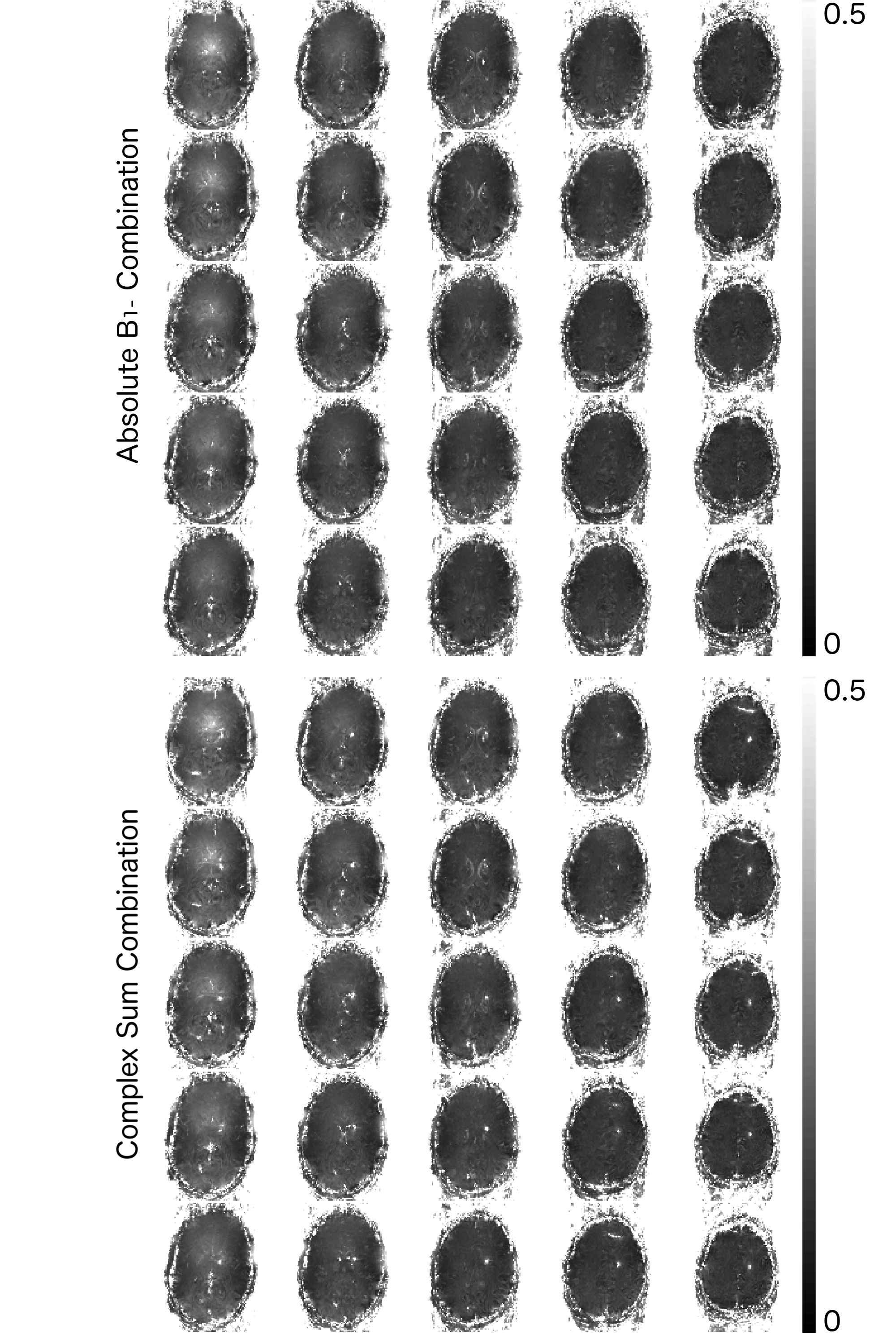
Temporal SNR of the conventional combination was subtracted from the receiver sensitivity combination on a voxel-wise basis. The mean difference between the $$$B_1^-$$$ combination and standard coil combination was 0.0665±1.2489. This was further validated using a Student’s t-test that had a significance value of p<10-10. The same subtraction was completed for phase standard deviation and the difference was -0.0087±0.1383 radians. This was also subjected to a Student’s t-test and the p-value of p<10-10 was found. In addition, Figure 3 shows the absolute $$$B_1^-$$$ combination does not produce any singularities in the brain opposed to a default complex sum which is the conventional combination for phase.Discussion
The lack of phase singularity in the EPI presented shows the immediate positive effect of scaling with a spatially varying $$$B_1^-$$$ profile. There was also a significant decrease in temporal phase standard deviation. Finally, an improvement is shown in tSNR compared to sum-of-squares. This method can be applied to any acquisition allowing for improved SNR in magnitude and phase.Conclusions
The ability to estimate $$$B_1^-$$$ without a homogeneous receive coil has immediate applications to future research. Current estimations using a homogeneous receive coil are still relative to that coil which has a unique $$$B_1^-$$$ profile that may not be homogeneous. By using the Helmholtz equations an absolute $$$B_1^-$$$ profile is found which allows for complete removal of the $$$B_1^-$$$ profile from the resulting images.Acknowledgements
No acknowledgement found.References
1 Curtis, A, Gilbert, K, Klassen, L, et al. Slice-by-slice B1+ shimming at 7 T. Magn Reson Med. 2012;68(4):1109–1116
2. Roemer P, Edelstein W, Hayes C, et al. The NMR phased array. Magn Reson Med. 1990;16(2):192-2253.
Figures