5068
Partial volume effect correction for surface-based cortical mapping1NeuroPoly Lab, Institute of Biomedical Engineering, Polytechnique Montreal, Montreal, QC, Canada, 2Athinoula A. Martinos Center for Biomedical Imaging, Charlestown, MA, United States, 3Montreal Health Institute, Montreal, QC, Canada, 4Harvard Medical School, Boston, MA, United States, 5Functional Neuroimaging Unit, CRIUGM, Université de Montréal, Montreal, QC, Canada
Synopsis
Partial Volume Effect (PVE) hampers the accuracy of studies aiming at mapping MRI signal in the cortex due to the close proximity of adjacent white matter (WM) and cerebrospinal fluid (CSF). The proposed framework addresses this issue by disentangling the various sources of MRI signal within each voxel, assuming three classes (WM, gray matter, CSF) within a small neighbourhood. MRI scans of 17 healthy subjects suggest robust estimations of PVE, allowing accurate extraction of MRI metrics using surface-based analysis. This method can be particularly useful for probing pathology in outer or inner cortical layers, which are subject to strong PVE with adjacent CSF or WM.
Purpose
Surface-based analysis is a popular method for mapping the MRI signal in the cortex, and for studying the healthy and pathological gray matter (GM) [1], [2]. However, given an average cortical thickness of ~2-3 mm [3] and a typical MR resolution of 1mm isotropic, many voxels in the cortex are juxtaposed with the white matter (WM) and the cerebrospinal fluid (CSF), yielding partial volume effect (PVE). As a result, the corresponding signal may be a combination of the unmixed values of adjacent tissues, which can lead to inaccurate quantification of the MRI signal in a desired region [4]. Here, we propose a framework that estimates the partial volume and determines the unmixed value of each hybrid voxel using least squared regression modeling.Methods
Data acquisition and pre-processing: 17 healthy subjects were scanned at 3T using the multi-echo MPRAGE sequence (1mm isotropic, TR/TI=2530/1100 ms, TE=[1.15, 3.03, 4.89, 6.75] ms). Pial and white matter (WM) surfaces were computed using Freesurfer [5].
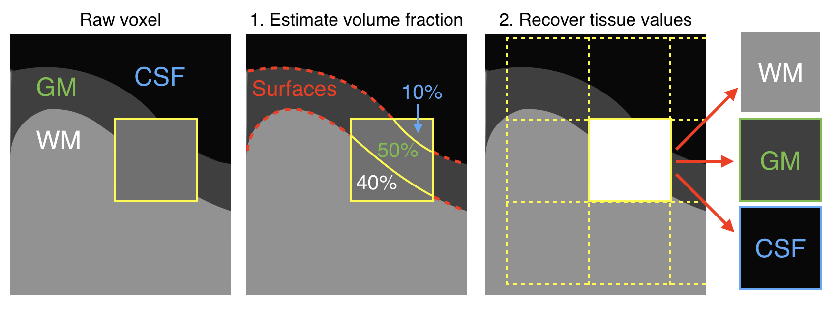
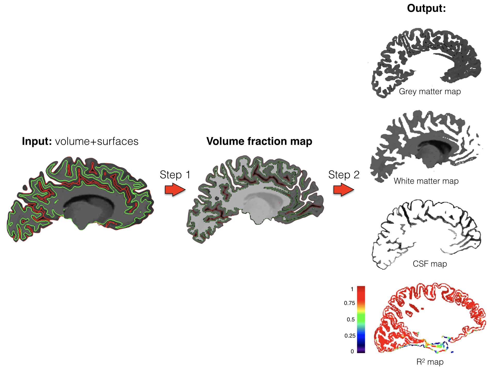
PVE estimation: Inputs are: the volume to correct, the WM-GM surface and the GM-CSF surface. Two automatic steps are performed.
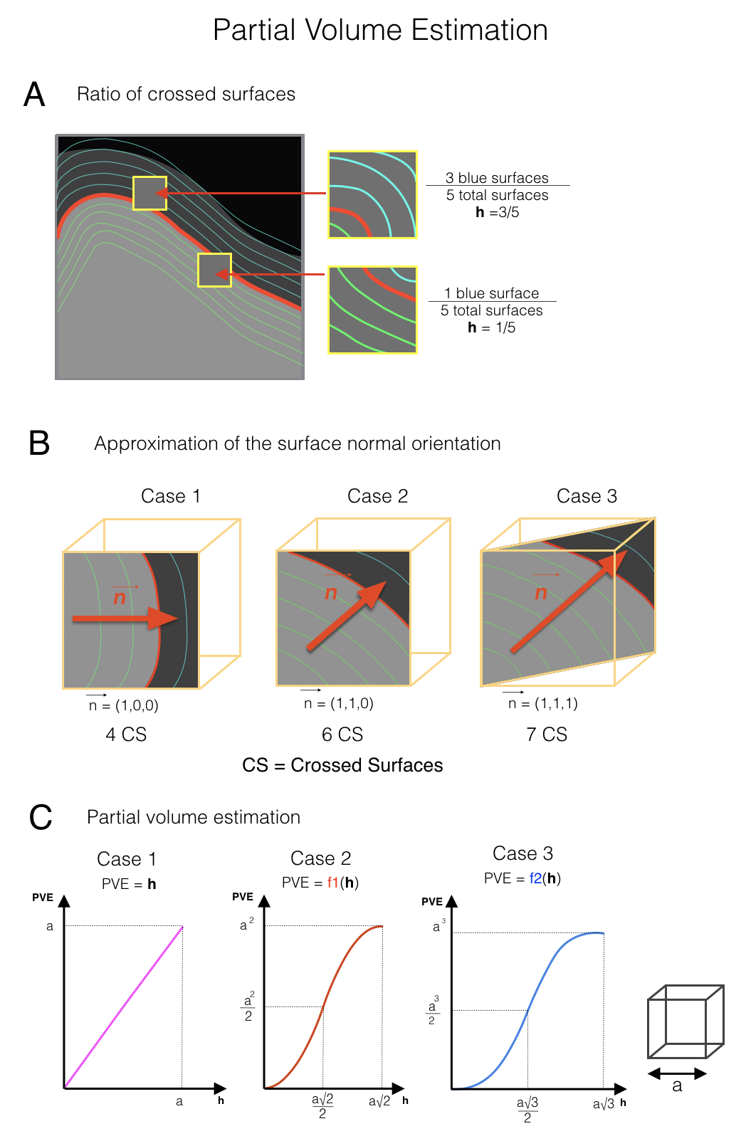
Step 1: Partial volume estimation (Fig 1): The tissue fraction in every mixed voxel is estimated as follows: 10 expanded surfaces (Fig 2) are created (5 in each side of the original surface, spaced with a 0.3mm gap) and the number of expanded surfaces intersecting each mixed voxel is calculated. Then, the ratio of surfaces crossed in one side out of the total crossed surfaces gives a first approximation of the volume in the exterior compartment (Fig 2A). The total number of surfaces crossing a voxel provides an approximation of the voxel orientation with respect to the normal of the surface (Fig 2B). This voxel orientation is used to refine the partial volume approximation (Fig 2C).
Step 2: Determination of the unmixed values (Fig 1 right.). Unmixed values of each tissue present in the voxel are determined using a least square estimation. Each intensity value in a voxel is assumed to be a weighted sum of the “true” tissue values (GM, WM and CSF) [6], where the weights are the volume fractions calculated earlier. For each voxel intersected by surfaces, the fraction of tissues in the neighboring voxels (3x3x3) are taken into account to solve the linear system with a least square estimation [7]: $$β= (X^{T}X)^{-1}X^{T}y$$
In which the unknown β is the vector of the unmixed signals, the weights X are the volume fractions for each tissue, and y contains the native voxels values.
Goodness-of-fit assessment: R-squared coefficients assess the robustness of each voxel’s linear estimation. Only voxels with R-squared>0.8 are kept in the output volumes (the threshold can be adjusted by the user).
Outputs: This framework outputs a set of 3 volumes, respectively containing the unmixed voxels values of each compartments: WM, GM and CSF (Fig 3).
Results
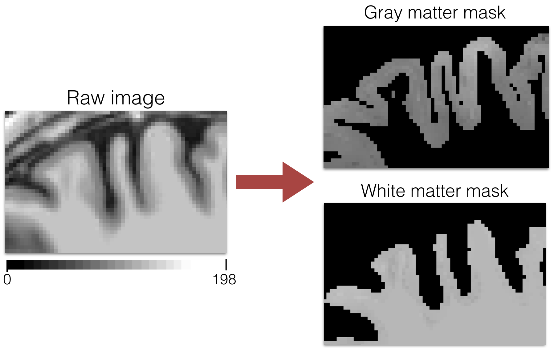
Out of the 17 subjects tested, 63.4% of the fitted voxel showed an R-square coefficient above 0.9 and for 87.7% of the voxels above 0.8. In the cortical ribbon, the average number of voxels not subject to PVE (i.e., GM fraction = 1) was 103k while the average number of voxels subject to PVE (GM fraction ∈]0, 1[) was 249k. Within the 249k voxels, 216k showed an unmixed estimation with R-squared>0.8, resulting in an increase of 209% of exploitable voxels for further cortical studies. Fig 4 shows an example of the GM and WM masks next to the original image.Discussion/Conclusion.
A method to estimate the fraction of partial volume and to recover the unmixed pixel values was presented. This method allows for more accurate extraction of MRI metrics using surface-based ROIs, and can be particularly useful for probing cortical demyelination in outer layers of the cortex, that are subject to strong partial volume with the CSF. Further validation is required on simulations and downsampled data. The framework is compatible with Freesurfer and is made available for public download at https://github.com/neuropoly/partial_volume_correction.Acknowledgements
We would like to thank Doug Greve & Bruce Fischl for sharing helpful scripts. This study was supported by the National Institute of Health [NIH R01NS078322-01-A1], the Canadian Institute of Health Research (CIHR FDN-143263), the Fonds de Recherche du Québec - Santé (FRQS 28826), the Fonds de Recherche du Québec - Nature et Technologies (FRQNT 2015-PR-182754), Quebec Bio-Imaging Network (QBIN), the Natural Sciences and Engineering research Council of Canada (NSERC), the Canada Research Chair.References
[1] C. Mainero et al., “In vivo imaging of cortical pathology in multiple sclerosis using ultra-high field MRI,” Neurology, vol. 73, no. 12, pp. 941–948, Sep. 2009.
[2] R. Turner, A.-M. Oros-Peusquens, S. Romanzetti, K. Zilles, and N. J. Shah, “Optimised in vivo visualisation of cortical structures in the human brain at 3 T using IR-TSE,” Magn. Reson. Imaging, vol. 26, no. 7, pp. 935–942, Sep. 2008.
[3] C. Hutton, E. De Vita, J. Ashburner, R. Deichmann, and R. Turner, “Voxel-based cortical thickness measurements in MRI,” Neuroimage, vol. 40, no. 4, pp. 1701–1710, May 2008.
[4] M. A. González Ballester, A. P. Zisserman, and M. Brady, “Estimation of the partial volume effect in MRI,” Med. Image Anal., vol. 6, no. 4, pp. 389–405, Dec. 2002.
[5] B. Fischl et al., “Automatically Parcellating the Human Cerebral Cortex,” Cerebral Cortex, vol. 14, pp. 11–22, 2004.
[6] H. S. Choi, D. R. Haynor, and Y. Kim, “Partial volume tissue classification of multichannel magnetic resonance images-a mixel model,” IEEE Trans. Med. Imaging, vol. 10, no. 3, pp. 395–407, 1991.
[7] C. L. Lawson and R. J. Hanson, Solving Least Squares Problems. SIAM, 1995.
Figures