5063
Visualization of Cardiac and Respiratory Pressure Gradient of Cerebrospinal Fluid Based on Asynchronous Two-Dimensional Phase Contrast Imaging1Graduate School of Engineering, Tokai University, Hiratshuka, Kanagawa, Japan, 2Graduate School of Science and Technology, Tokai University, Hiratsuka, Kanagawa, Japan, 3Department of Neurosurgery, Tokai University School of Medicine, Isehara, Kanagawa, Japan
Synopsis
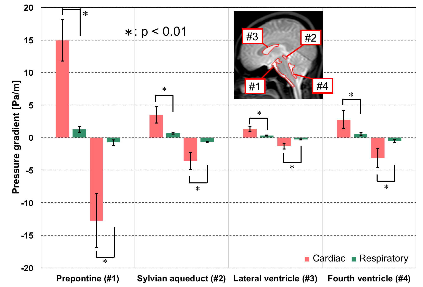
To visualize the distribution of the pressure gradients of the cardiac- and respiratory-driven cerebrospinal fluid (CSF), asynchronous two-dimensional phase-contrast velocity imaging was performed in 9 healthy subjects. The pressure gradients were calculated by the Navier–Stokes equations after the total CSF motion was classified into either cardiac or the respiratory components in the frequency domain. In the prepontine, the pressure gradients in the caudal-to-cranial direction were 14.9 ± 3.17 Pa/m for cardiac components and 1.28 ± 0.46 Pa/m for respiratory components; the cardiac pressure gradient was also significantly larger than the respiratory pressure gradient in other regions.
Introduction
In our previous work, the cardiac- and respiratory-driven cerebrospinal fluid (CSF) motions were separated, and the power ratio between them was visualized.1 In addition, the pressure gradient of the total CSF motion was visualized to demonstrate the difference between healthy subjects and patients with hydrocephalus.2 Based on the results of our previous study, in this study, the pressure gradients of the cardiac- and respiratory-driven CSF velocities were obtained and evaluated to assess the spatial distribution of the motive force of CSF.Material and methods
In total, 9 healthy subjects (8 males and 1 female, 24 ± 4 years) were instructed to a 6-sec respiratory cycle using audio guidance. Cardiac pulsation and respiration were recorded using electrocardiography (ECG) and a bellows pressure sensor, respectively. Asynchronous two-dimensional phase-contrast (2D-PC) imaging with steady-state free precession was performed at 3T (flow direction: foot–head (FH); data points: 256; TR: 6.0 msec; TE: 3.9 msec; field of view: 28 × 28 cm2; velocity encoding: 10 cm/sec; acquisition matrix: 89 × 128; reconstruction matrix: 256 × 256; slice thickness: 7 mm; frame rate: 4.6 images/sec; temporal resolution: 217 ms).
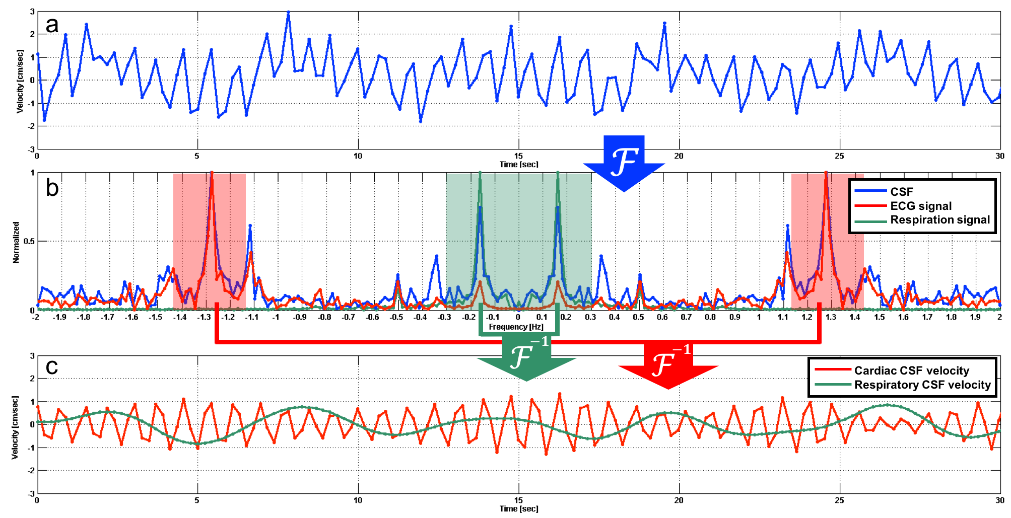
The total CSF velocity (Figure 1a) of each subject was Fourier-transformed into a spectrum (the blue line in Figure 1b) and compared with the ECG (the red line in Figure 1b) and respiratory (the green line in Figure 1b) spectra obtained from the log data. Then, the corresponding ± 0.15 Hz frequency bands around the peaks of the ECG and respiratory spectra were extracted and inversely transformed to have cardiac and respiratory CSF velocities (Figure 1c). After, the pressure gradients were calculated along the cranio-caudal region as follows:
$$${\bf\triangledown}{P}=-\rho(\frac{\bf\partial v}{\partial t}+{\bf{v}\cdot\triangledown{v}})+\mu\cdot{\bf\triangledown^{2}v}$$$ (1),
where P is the pressure, $$$\bf v$$$ is the velocity, t is the time, ρ is the fluid density (1.007 × 10³ kg/m3 for CSF), and μ is the dynamic viscosity (1.1 × 10⁻³ Pa·s for CSF). The pressure gradients were then depicted voxel by voxel; voxels containing major arteries or veins were removed manually.
To quantify the pressure gradient, the following four regions of interest (ROIs) were selected: (1) the prepontine, (2) the sylvian aqueduct, (3) the lateral ventricle, and (4) the fourth ventricle.3 The averages of the peak positive (caudal-to-cranial) and negative (cranial-to-caudal) pressure gradients were plotted for each subject.
Results
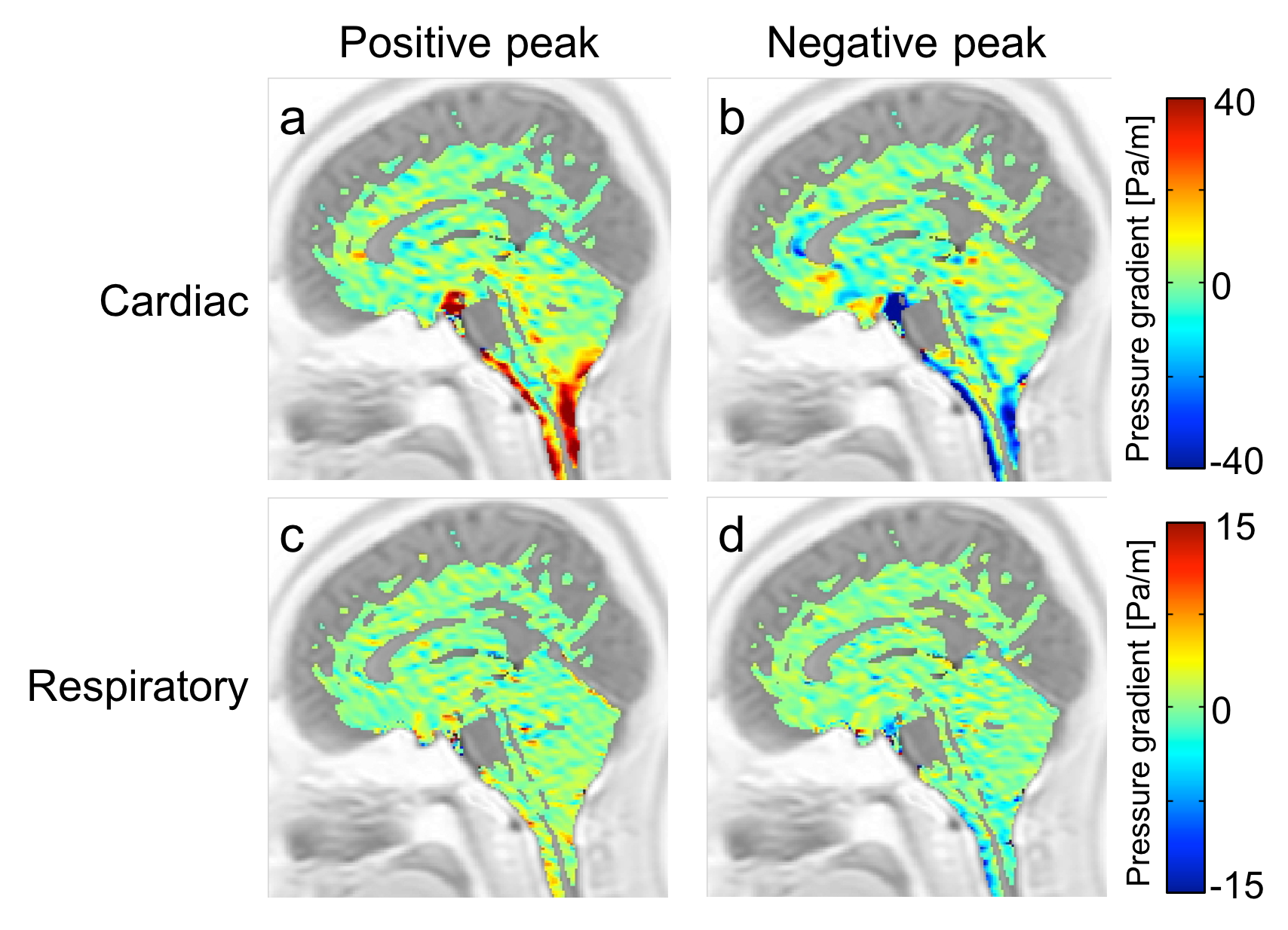
Figure 2a shows a typical cardiac pressure gradient image at the positive peak, while Figure 2b represents the same at the negative peak. Figures 2c and 2d present the same, but for the respiratory components. Figure 3 depicts the results of the quantitative analysis of the cardiac and respiratory pressure gradients. At all the ROIs, significant differences (p < 0.01) were found between the cardiac and respiratory pressure gradients.Discussion
This study was conducted to visualize the cardiac- and respiratory-based motive force of CSF in healthy subjects. As shown in Figure 2, the cardiac-driven pressure gradient was higher in the prepontine than the respiratory-driven pressure gradient. Our pressure gradients were smaller than those found in previous works by about one-tenth.2,3 This may be because our results separated the cardiac- and respiratory-driven motions rather than displaying the total motion, because CSF velocity observations were only made in the FH direction, or because the spatiotemporal resolution was low due to acquisition acceleration, which could have led to a degradation in the calculation’s accuracy.
Nevertheless, the cardiac-driven pressure gradient was consistently higher than the respiratory-driven pressure gradient in both directions (Figure 3). The size of the cardiac component at the prepontine was likely caused by the pulsating artery around the prepontine. Although the prepontine links with the sylvian aqueduct and the fourth ventricle, the cardiac-driven pressure gradients decreased possibly because of the compliance of the intracranial CSF pathway, which may have obstructed or absorbed pressure.
The pressure gradients at the lateral ventricle were lower. CSF flow becomes turbulent in the lateral ventricles, meaning that the pressure gradient was unclear. The significantly larger pressure gradient of the cardiac pulsation presented here does not mean a larger displacement of CSF.4Conclusion
The separation of the cardiac- and
respiratory-driven pressure gradients of CSF based on asynchronous 2D-PC velocity
imaging was demonstrated. The cardiac pressure gradients in the intracranial ROIs
of healthy subjects were significantly higher than the respiratory pressure
gradients. The primary drawbacks of the present technique were the low
spatiotemporal resolutions used and the one-directional velocity encoding used to
accelerate the asynchronous data sampling. A sophisticated and rapid sampling
technique, such as sparse k-space sampling, should be employed in future work.
Acknowledgements
The authors thank Prof. Yutaka Imai, Mr. Tomoaki Horie, and Mr. Nao Kajihara, for their assistance with MRI.References
1. Sunohara S, Yatsushiro S, Takizawa K et al. Investigation of driving forces of cerebrospinal fluid motion by power and frequency mapping based on asynchronous phase contrast technique. Proc IEEE EMBC. 2016;1232-1235.
2. Matsumae M, Hirayama A, Atsumi H et al. Velocity and pressure gradients of cerebrospinal fluid assessed with magnetic resonance imaging. J Neurosurgery. 2014;120(1):218-27.
3. Hayashi N, Matsumae M, Yatsushiro S et al. Quantitative analysis of cerebrospinal fluid pressure gradients in healthy volunteers and patients with normal pressure hydrocephalus. Neurol Med Chir (Tokyo). 2015;55(8):657-62.
4. Yamada S, Miyazaki M, Yamashita Y et al. Influence of respiration on cerebrospinal fluid movement using magnetic resonance spin labeling. Fluids Barriers CNS. 2013;10(1):36.
Figures