4963
Spatially-sensitive model for detection of prostate cancer on multiparametric MRI1Center for Magnetic Resonance Research, University of Minnesota, Minneapolis, MN, United States, 2Division of Biostatistics, School of Public Health, University of Minnesota, Minneapolis, MN, 3Department of Urologic Surgery, Institute of Prostate and Urologic Cancers, University of Minnesota, Minneapolis, MN, United States, 4Department of Radiology, University of Minnesota, Minneapolis, MN, United States
Synopsis
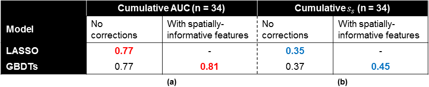
A novel predictive model of prostate cancer (PCa) on multiparametric MRI was developed that takes into account the spatial distribution of PCa within the prostate and the spatially-autocorrelated nature of mpMRI data. The performance of the proposed model was compared to the LASSO-based model we previously described on 34 PCa cases using both voxel-wise metrics (AUC) and slice-wise metrics ($$$s_s$$$) we recently developed. The proposed model achieved superior predictive performance both in terms of AUC (0.81 vs 0.77) and $$$s_s$$$ (0.45 vs. 0.35) over the 34 cases, with significant improvements for the majority of cases.
Rationale
There has been interest recently in using quantitative multiparametric MRI (mpMRI) for detecting prostate cancer (PCa) and assessing the clinical significance of disease. One major focus is the development of computational models that use mpMR data to make predictions about PCa status.1-4 Previously, we described a LASSO-based 5-parameter model that demonstrated superior voxel-wise classification performance as compared to any single MR parameter.5 Here, we describe a novel model that improves upon our existing work by employing a machine-learning framework with corrections that address the spatial effects present in the mpMR data.Methods
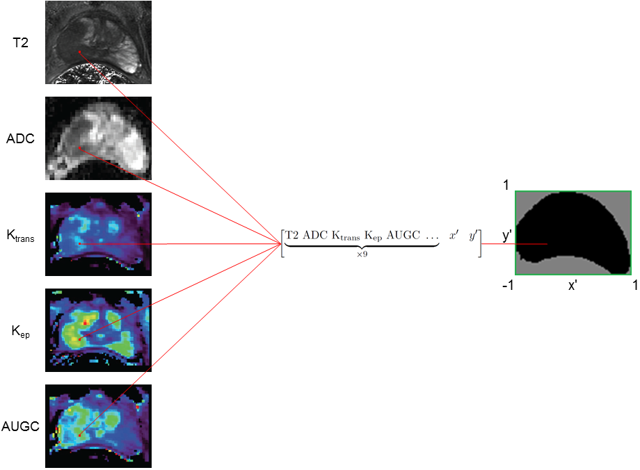
Data used for model development were acquired following protocols we previously described.5 Briefly, patients received mpMR scans at 3T under an approved IRB protocol. Histopathology data were obtained through processing of post-surgical ex vivo prostate specimens from patients that underwent radical prostatectomy. MR slices containing index lesions were then co-registered to the pathology data. 34 patient cases containing 46 slices of interest and 100,000+ voxels were included for modeling. For each voxel, its mpMR values were used as modeling inputs (features), while its cancer status (label) was used as the ground truth. The five mpMR parameters used for modeling were the tissue T2 value, ADC value, and three DCE-MRI parameters derived from pharmacokinetic curve fitting (Ktrans, Kep, AUGC).
In our previous work, it was implicitly assumed that voxels could be treated as if they were drawn from the same joint probability distribution, meaning that the expected parameter values and PCa likelihood for a given voxel is the same as that of any other voxel. However, this assumption is untrue because expected parameter values and PCa likelihood for a given voxel depend on those of its neighbors and also vary among the anatomical regions of the prostate (highest likelihood in the peripheral zone).6
To account for these spatial dependencies, the features were augmented in two ways. First, the relative xy-positions of each voxel were included as additional features. This provides information about the location of the voxel within the prostate, which provides a surrogate for anatomical location without the need to perform segmentation. Second, mpMR parameters of all immediately adjacent neighbors of a voxel were included as additional features. This is a simple way to incorporate spatial autocorrelation into the model. Altogether, each voxel was associated with 47 features (Fig. 1).
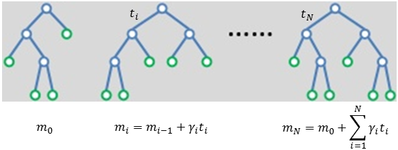
The machine-learning algorithm used to perform classification is gradient-boosted decision trees (GBDTs), which was implemented in Python through the Xgboost package.7 It is an ensemble learning approach that starts with a weak decision tree and iteratively improves its fit to the training data (boosting). The final prediction is then a weighted sum of the predictions of all of the decision trees (Fig. 2). This algorithm was primarily selected for its fast training times and superior results in many machine-learning competitions.7
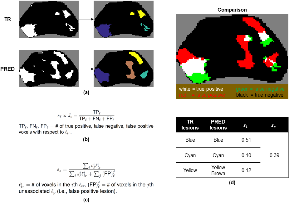
The performance of the proposed GDBTs-based model vs. that of the LASSO-based model we previously described was compared in two ways. Area under the receiver operating curve (AUC), a balanced measure of voxel-wise sensitivity and specificity, was calculated for all cases. A slice-wise metric based on the overlap between distinct foci of PCa (or lesions) in the prediction and ground truth ($$$s_s$$$) that we recently developed (Fig. 3) was also calculated for all cases.
Results
For both models, a case-based leave-one-out cross-validation scheme was used to train and assess performance; for a given PCa case, the models were first trained using the data from the other 33 cases, then evaluated on the case itself. Table 1 shows the cumulative AUC and $$$s_s$$$ across all cases for both models.
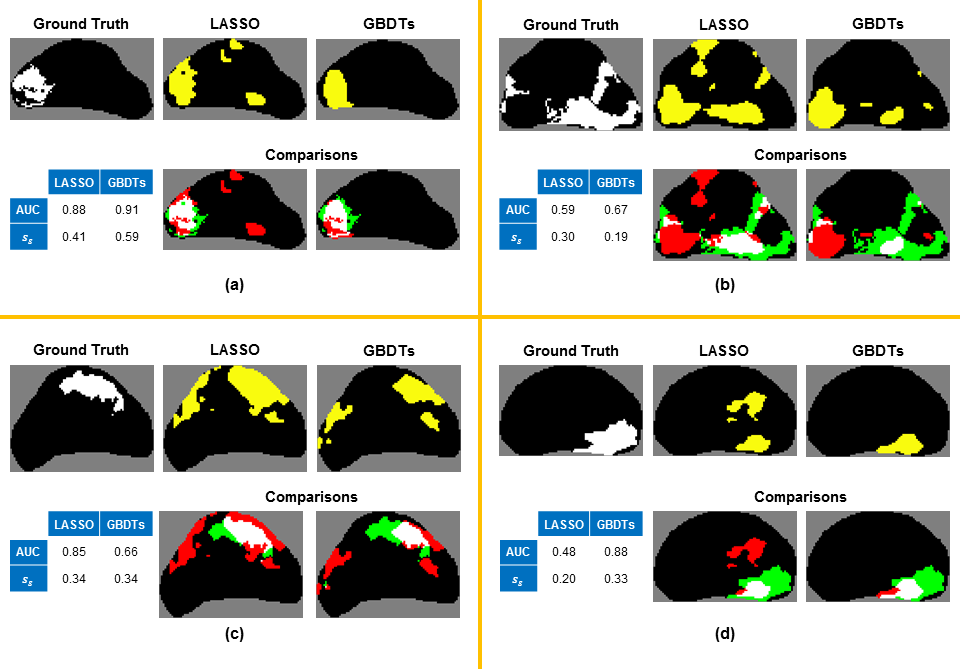
In terms of AUC, the proposed model performed significantly better (ΔAUC ≥ 0.05) on 19/34 cases. Similarly, in terms of $$$s_s$$$, the proposed model performed significantly better (Δ$$$s_s$$$ ≥ 0.1) on 25/34 cases. Although both metrics were generally in agreement, Figure 4 illustrates representative prediction maps for specific slices in which AUC and $$$s_s$$$ differed between the two models. It appeared that the new evaluation metric $$$s_s$$$ is superior to AUC at accurately reflecting the differences in the quality of predictions.
Discussion
Incorporating features that account for the spatial characteristics of mpMRI data improved predictive performance as measured by both voxel-wise and lesion-wise metrics. However, as Figure 4 illustrates, there exists significant variation in model performance among different cases. This is most likely explained by differences in the joint probability distribution of mpMR parameters and PCa likelihood among different patients and different grades of PCa, which we plan to address in future work.Acknowledgements
Supported by: NCI R01 CA155268, NIBIB P41 EB015894, DOD/PCRP W81XWH-15-1-0477, MN-REACH.References
1. Chan I, Wells W, 3rd, Mulkern RV, Haker S, Zhang J, Zou KH, Maier SE, Tempany CM. Detection of prostate cancer by integration of line-scan diffusion, T2-mapping and T2-weighted magnetic resonance imaging; a multichannel statistical classifier. Med Phys. 2003;30(9):2390-8.
2. Artan Y, Haider MA, Langer DL, van der Kwast TH, Evans AJ, Yang Y, Wernick MN, Trachtenberg J, Yetik IS. Prostate cancer localization with multispectral MRI using cost-sensitive support vector machines and conditional random fields. IEEE transactions on image processing: a publication of the IEEE Signal Processing Society. 2010;19(9):2444-55. doi: 10.1109/tip.2010.2048612.
3. Tiwari P, Kurhanewicz J, Madabhushi A. Multi-kernel graph embedding for detection, Gleason grading of prostate cancer via MRI/MRS. Medical image analysis. 2013;17(2):219-35. doi: 10.1016/j.media.2012.10.004.
4. Litjens G, Debats O, Barentsz J, Karssemeijer N, Huisman H. Computer-aided detection of prostate cancer in MRI. IEEE Trans Med Imaging. 2014;33(5):1083-92. doi: 10.1109/tmi.2014.2303821.
5. Metzger GJ, Kalavagunta C, Spilseth B, Bolan PJ, Li X, Hutter D, Nam JW, Johnson AD, Henriksen JC, Moench L, Konety B, Warlick CA, Schmechel SC, Koopmeiners JS. Detection of Prostate Cancer: Quantitative Multiparametric MR Imaging Models Developed Using Registered Correlative Histopathology. Radiology. 2016;279(3):805-16. doi: 10.1148/radiol.2015151089.
6. Kumar V, Abbas AK, Aster JC. Robbins & Cotran Pathologic Basis of Disease. 9th ed. Philadelphia: Elsevier Saunders; c2015. 1408 p.
7. Chen T, Guestrin C. XGBoost: A Scalable Tree Boosting System. Proceedings of the 22nd ACM SIGKDD International Conference on Knowledge Discovery and Data Mining. 2016:785-94. doi: 10.1145/2939672.2939785.
8. Levandowsky M, Winter D. Distance between Sets. Nature. 1971;234(5323):34-35. doi: 10.1038/234034a0.
Figures