4797
Modified Dispersion Model in Prostate Dynamic Contrast-Enhanced MRI1Radiological Sciences, University of California, Los Angeles, Los Angeles, CA, United States, 2Radiology, University of California, Los Angeles, Los Angeles, CA, United States
Synopsis
The dispersion imaging has shown great promise in prostate DCE-MRI, but there still exist practical limitations due to the complex model fitting. We describe a modified dispersion model to overcome these limitations by adapting a simple dispersion factor into the existing population-averaged arterial input function. We use the regions of interest, derived from the histological analysis, to evaluate both the quality of the model fitting and the ability of DCE-MRI parameters to delineate between cancerous and normal prostate tissues using 25 prostate patient cases available with the whole-mount histopathology.
Introduction
Quantitative dynamic contrast-enhanced MRI (DCE-MRI) has great potential to improve the specificity in the diagnosis of prostate cancer (PCa). The dispersion imaging by DCE-MRI has shown great promise in prostate cancer [1], but there still exist practical limitations due to the complex model fitting. In this work, we describe a modified dispersion model to overcome these limitations by adapting a simple dispersion factor. We use the regions of interest (ROIs), derived from the histological analysis, to evaluate both the quality of the model fitting and the ability of DCE-MRI parameters to delineate between cancerous and normal prostate tissues using 25 prostate patient cases available with the whole-mount histopathology.Methods
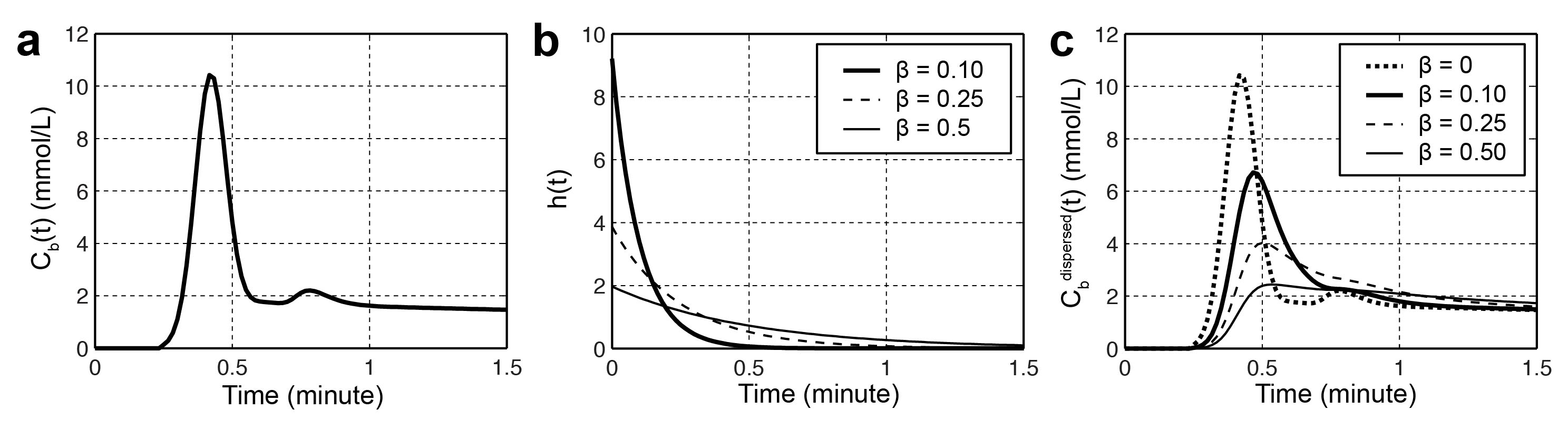
The recently proposed dispersion imaging [1] has shown the microvascular architectures of PCa can be characterized without need for a separate arterial input function (AIF) estimation. However, the proposed dispersion model sometimes suffers from unstable results because of possible local minima in the model fitting. To overcome this limitation, we have modified the dispersion model by introducing a simple dispersion factor β for a given AIF, Cb(t) [2]. The modified dispersion model can be described as a convolution with a vascular transport function h(r,t) at a position r from Cb(t) (Fig 1):
Cbdispersed(r,t) = Cb(t) * h(r,t), where h(r,t) = 1/β(r) e (-t/β(r)).
In the modified dispersion model, we used the Parker AIF [3] for Cb(t), and β is directly fitted to time-concentration curves (TCCs) along with Ktrans and kep in the standard Tofts model, limiting the number of free parameters in the model fitting to avoid the possible local minima.
DCE-MRI data was acquired in 25 patients who later underwent radical prostatectomy on Siemens 3T systems. The DCE-MRI protocol consisted of a 3D spoiled gradient echo acquisition with the temporal resolution of 4.2s, TE of 1.5ms and TR of 3.9ms. T1 maps were measured using the variable flip angle (VFA) imaging with a set of flip angles (2°, 5°, 10°, and 15°) for the conversion of signal intensity to contrast agent concentration. The histopathological analysis was meticulously carried out such that accurate correlation could be achieved between cancerous regions of prostate identified from pathology and the imaging slices. ROIs containing cancerous tissue derived from the histology were drawn onto the corresponding imaging slices. Reference ROIs in normal transition zone (TZ) tissue were used for comparison to assess how well the modeled parameters delineate between cancerous and normal TZ tissue.
We compared the modified dispersion model with three population-averaged AIFs, including Parker [3], Weinmann [4], and Fritz-Hans [5], using the standard Tofts model [6]. The residual errors were measured by a sum of the squared residual values during the 90 sec initial contrast uptake (the gray area in Fig 2). β(r) was grouped into two classes, low- and high-dispersion, using the Gaussian mixture model, and the normalized low-dispersion map was multiplied to the dispersion-based Ktrans to create the dispersion-weighted Ktrans. The dispersion-weighted Ktrans and Ktrans with three different AIFs were evaluated in normal TZ and PCa ROIs over the cohort of 25 patients.
Results and Discussion
A representative example of the residual errors in three different positions is shown in Fig 2. The Parker AIF has a good fitting quality in a cancerous region (Fig 2b and d) but a poor fitting quality in normal TZ (Fig 2c), while the modified dispersion model achieves a great fitting quality in all areas by adapting different dispersion factors, as also shown in Fig 3. Table 1 contains the mean and standard deviation of the residual errors in PCa, normal TZ and whole prostate glands, and the modified dispersion model achieves the minimum residual errors in all ROIs. The parameters in PCa and normal TZ also show that the modified dispersion model has greatly achieved the improved contrast between PCa and normal TZ. The results support the hypothesis that angiogenesis causes increased perfusion and the capillary walls of cancerous tissue and more permeable than normal tissue. Future work includes analyzing more patient data, associating with histological findings such that a range of ‘normal’ and ‘potentially cancerous’ values can be identified for each region to aid the use of DCE-MRI in both diagnosis and active surveillance.Conclusion
We showed the modified dispersion model could successfully achieve the minimal model fitting error and improved contrast between prostate cancer and normal tissue.Acknowledgements
This study is supported by Siemens Healthcare.References
1. Kuenen MPJ, Saidov T a, Wijkstra H, Mischi M: Contrast-ultrasound dispersion imaging for prostate cancer localization by improved spatiotemporal similarity analysis. Ultrasound Med Biol 2013, 39:1631–41.
2. Calamante F, Gadian DG, Connelly A: Delay and dispersion effects in dynamic susceptibility contrast MRI: simulations using singular value decomposition. Magn Reson Med 2000, 44:466–73.
3. Parker GJM, Roberts C, Macdonald A, et al. Experimentally-derived functional form for a population-averaged high-temporal-resolution arterial input function for dynamic contrast-enhanced MRI. Magn Reson Med. 2006;56(5):993-1000..
4. Weinmann HJ, Laniado M, Mützel W. Pharmacokinetics of GdDTPA/dimeglumine after intravenous injection into healthy volunteers. Physiol Chem Phys Med NMR. 1984;16(2):167-172.
5. Fritz-Hansen T, Rostrup E, Larsson HB, Søndergaard L, Ring P, Henriksen O. Measurement of the arterial concentration of Gd-DTPA using MRI: a step toward quantitative perfusion imaging. Magn Reson Med. 1996;36(2):225-231.
6. Tofts PS, Brix G, Buckley DL, Evelhoch JL, Henderson E, Knopp M V, Larsson HB, Lee TY, Mayr N a, Parker GJ, Port RE, Taylor J, Weisskoff RM: Estimating kinetic parameters from dynamic contrast-enhanced T(1)-weighted MRI of a diffusable tracer: standardized quantities and symbols. J Magn Reson Imaging 1999, 10:223–32.
Figures