4758
Automated 4D Flow Conservation Utilizing Adjacency MatricesCarson Anthony Hoffman1, Gabe Shaughnessy1, and Oliver Wieben1
1Medical Physics, University of Wisconsin Madison, Madison, WI, United States
Synopsis
4D flow magnetic resonance imaging (MRI) can provide comprehensive information on vessel anatomy and hemodynamics for complex vessel system. Adjacency matrices are often used in computer science to help simplify complex graphs into a binary encoded matrix. The adaptation of adjacency matrices to 4D flow MRI can help reduce the complexity for analysis by structuring the data into an efficient binary matrix. One application of this new analysis method allows for flow conservation to be completed for complex volumes at all junctions. The conservation of flow at every junction can then be used to find segments of potential erroneous measurements.
Purpose
4D flow magnetic resonance imaging (MRI) allows for the encoding of complex velocity fields over a cardiac cycle. Post processing of 4D flow MRI datatsets can be time consuming and the identification of ‘problem zones’ such as velocity aliasing or intravoxel dephasing from complex flow can be problematic, especially for large imaging volumes and high vascular density such as in cranial and hepatic scans. The risk of missing corrupt data or misinterpreting results is especially high for less experienced users as 4D flow analysis finds more widespread use. Here we introduce the concept of an automated algorithm to identify suspicious vessel segments using the idea of flow conservation throughout the complete vessel network with adjacency matrices. This method has the potential to identify vessel branches where flow conservation is violated and thereby reduce accidental misinterpretation of 4D flow data.Methods
Adjacency matrices are commonly used in graph theory to help organize complex graphs into a structured vertices matrix. The adjacency matrix uses binary labeling to encode the connectivity of all the vertices in a simple and efficient manner as shown in Fig 1. The size of the adjacency matrix is a square matrix with a row and column length equal to the number of vertices. By altering the encoding parameter from vertices to vessel branch segments, we encode complex vessel connectivity into a binary matrix. Due to the directionality of flow, the adjacency matrix becomes asymmetric in our adapted version. The parallel between a vertex and vessel branch adjacency matrix approach can be seen in Fig1. The row of the matrix indicates the vessel branch. The 1’s column location in the associated row indicate which branches are connected to the current branch. Five cranial scans were completed for this study after IRB approval and providing consent. Imaging was performed on a clinical 3T scanner using 4D flow MRI with an undersampled radial acquisition, PC VIPR2. A vessel skeleton of the vasculature with labeled branches was automatically generated using a centerline algorithm Fig2. Subsequently, the average flow for each centerline point was calculated by generating an analysis plane perpendicular to the centerline and integrating velocity volumes over the vessel area., all with an in-house software tool (MATLAB 2015a). The average flow for each segment was represented by the mean of centerline flow values along that vessel segment near the center of each branch. Adjacency matrices were generated for the vascular tree and analyzed for flow consistency.Results
Automatic construction of adjacency matrices was successful in all of the presented cranial cases. Conservation of flow calculations for 3 locations in a single case are presented in Fig3. The percent error increased as the analyzed bifurcation moved from large proximal to smaller distal vessels. Percent errors in flow conservation ranged from ~1-10% for good flow conservation and from 11-55% where flow was not conserved as seen in Fig4. Mislabeled junctions due noisy or incomplete angiograms was minimal in this study. The processing needed to complete all conservation of flow measurements in a single case took less than 2 minutes.Discussion
We were able to show that quick flow conservation validation for junctions in complex vessel networks is possible using our adapted adjacency method. As the junctions moved from proximal to distal the vessel sizes decreased and the error increased accordingly. The increased error for smaller vessel was expected due to lower SNR and a high influence from the partial volume effect. The highest influence of error for this method is thought to be related primarily to vessel area calculations. Examples of some possible errors from incorrectly defined angiograms are shown in Fig5. Defining tolerance levels for incorrect flow conservation based upon junction location has yet to be completed. A comparison between different subjects was not completed in this study.Conclusion
We introduced a new scheme for automated consistency checks of flow measures in vascular trees and demonstrated its use in 5 cranial studies. The concept of adjacency matrices coupled with vessel segments can be utilized in 4D flow MRI to quickly provide feedback on data consistency and potential problem zones. Future work utilizing the adjacency matrix and uncertainty values of all vessel segments may allow for corrective flow algorithms to be applied. The levels of tolerable uncertainty related to flow, area, and velocity when applying the corrective flow algorithm will need to be investigated further.Acknowledgements
No acknowledgement found.References
1) E. Schrauben, et al J Magn Reson Imaging. 2015 Nov;42(5):1458-64 2) Johnson, K. M. et al Magnetic Resonance in Medicine. 2008; 60(6), 1329-1336.Figures
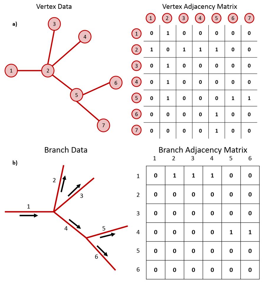
Figure 1: Adjacency
matrices are commonly used in graph theory to encode vertex data into a binary
matrix. a) An example vertex data orientation with its associated adjacency
matrix. b) Sample branch network similar to the structure of a) but with the
new branch encoded adjacency matrix applied. The arrows indicated the direction
of flow. Due to flows directional nature the adjacency matrix becomes
asymmetric.
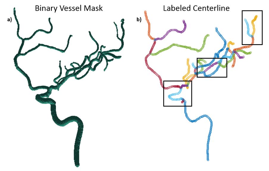
Figure 2: a) Left
carotid artery of subject #2 visualized as a surface shaded display. The automatically
labeled centerline tree with three junctions of interest for flow validation are
shown in b). The labeled centerline is color coded to give a better
representation of the number of segments and junctions. Each circle along the
centerline represents a measurement point.
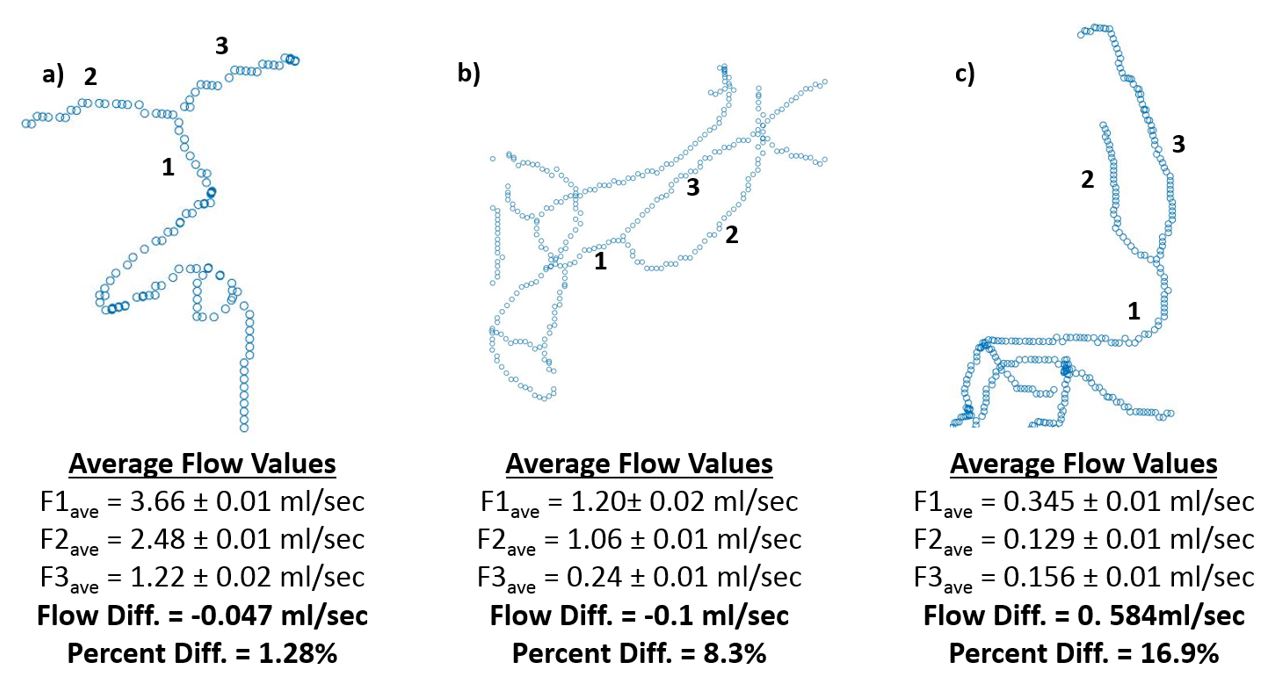
Figure 3: A zoomed
view centerline points of 3 of the 13 identified junctions are shown for
subject #2 along with flow in and out of the bifurcations. The 3 locations used are views of the boxed
regions in Figure 2. a) The most proximal bifurcation with largest vessel size
resulted in the lowest error when testing for consistency between inflow and
outflow (1.28%). c) The most distal
vessel and smallest vessel size resulted in the greatest error. b) Located
between a) and c) produced an error value between the error range of a) and c).
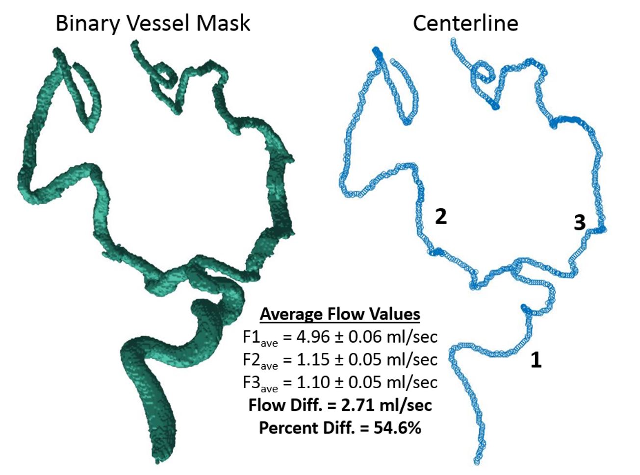
Figure 4: A clear
case where the automated segmentation failed to pick up all the major vessels
in the brain. The conservation of flow is not preserved in this case and
results in a large percent difference in average flow as expected.
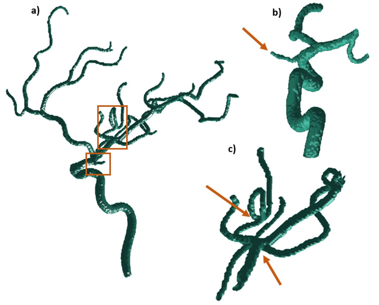
Figure 5: Right
carotid artery of subject #1. The automatically segmented arterial vascular
tree is visualized as a surface shaded display a) produced minimal areas of
incorrectly defined vessels for the presented case. A vessel spur due to noise
is indicated by the arrow in b). Vessel overlap (top arrow) and complex vessel
junctions (bottom arrow) shown in c) caused incorrect junction labeling.