4754
Semi-Automatic Ejection Fraction Calculation from Cardiac Low-Rank Tensor Images Based on Unsupervised Machine Learning1Biomedical Imaging Research Institute, Cedars-Sinai Medical Center, Los Angeles, CA, United States, 2Center for Biomedical Imaging Research, Department of Biomedical Engineering, School of Medicine, Tsinghua University, Beijing, People's Republic of China, 3Cedars-Sinai Heart Institute, Cedars-Sinai Medical Center, Los Angeles, CA, United States, 4Department of Bioengineering, University of California Los Angeles, Los Angeles, CA, United States
Synopsis
Calculation of the ejection fraction from cardiac cine MR images requires segmenting multiple images of the left ventricle. This process, which is often performed manually, is time-consuming and observer-dependent. In this work, an unsupervised machine learning algorithm, combining hidden Markov random field and optical flow, has been proposed to perform semi-automatic tissue segmentation on T1/T2-weighted low-rank tensor images that have a built-in feature space due to low-rank factorization performed during image reconstruction. The segmentation results then allow automatic EF calculation. Demonstrated results have higher efficiency and similar accuracy compared with manual segmentation, and were stable with respect to different initializations.
Purpose
Many clinically relevant cardiac measurements are based on the size or shape of segmented tissues derived from cardiac MR images. For example, ejection fraction (EF) is the fraction of outbound blood pumped from the heart with each heartbeat, which can be approximated by the shrinking percentage of the size of the left ventricle (LV) within a cardiac cycle. The traditional manual segmentation is inefficient and suffers from inter-observer variations. Some computer-assisted methods are based on the active contour model1,2, and often have difficulty with papillary features. Other methods are based on prior knowledge of the shapes and values3, and are therefore not robust to changing LV shapes and inter-subject variations. Here we propose a region-based semi-automatic method, taking advantage of the spatial and temporal continuity of tissues, as well as the built-in feature space provided by explicit-subspace low-rank imaging4,5, to segment different tissues with only a few clicks, obtaining EF and other volume-based cardiac assessments.Methods
Images were acquired using low-rank tensor-based cardiovascular MR (CMR) multitasking6, resulting in different T1/T2-weighted contrast images at different time points. In this way, it provides many features to uniquely identify a specific tissue. This imaging method was selected because the temporal subspace constraint at the foundation of low-rank tensor CMR multitasking also provides a convenient feature space for image segmentation, bypassing the need for feature extraction. By assuming the values in this feature space follow a Gaussian Mixture Model (GMM), we cluster the results according to the maximum a posteriori (MAP) criterion. A neighborhood potential term is incorporated to enforce the spatial and temporal continuity. Edges are preserved by disregarding the effect from neighboring voxels on a contour7. The resulting model is a hidden Markov random field (HMRF) model8 defined on a 3-D space (2 image dimensions and a time dimension depicting cardiac motion). Then the expectation-maximization (EM) algorithm9 is applied to solve the following optimization function.
$$\hat{\bf{Y}} =\arg\underset{\bf{Y}}{\min}\,\left[U(\bf{X}|\bf{Y} ;\Theta)+U(\bf{Y})\right]$$
where Y is the configuration of all clusters (i.e., tissues) that each voxel belongs to, X denotes the data in the feature space and Θ denotes the distribution parameter set (which is time-variant due to blood flow effects). The two potential terms represent neighborhood potential and probability potential respectively in the following form:
$$U(\bf{X}|\bf{Y};\Theta)=-\sum_{i} \log{P(\bf{x}_i|y_i;\Theta)}$$
$$U(\bf{Y})=\sum_{c \in C} V_c (\bf{Y})$$
where P is the Gaussian distribution probability, C denotes all the neighboring pairs and Vc(Y) denotes the potential on pair c. In order to more easily allow volumes to change size between successive frames, an optical flow10 algorithm was used to predict values of Y at neighboring times. Specifically, we estimate the velocity (vx, vy) at each voxel from black-blood images:
$$\left[\begin{matrix}\bf{I}_x^T\bf{I}_x & \bf{I}_x^T\bf{I}_y \\\bf{I}_x^T\bf{I}_y & \bf{I}_y^T\bf{I}_y\end{matrix}\right]\left[\begin{matrix}v_x \\v_y\end{matrix}\right]=-\left[\begin{matrix}\bf{I}_x^T\bf{I}_t \\\bf{I}_y^T\bf{I}_t\end{matrix}\right]$$
where Ix, Iy and It denote the corresponding derivative vectors.
Experiments
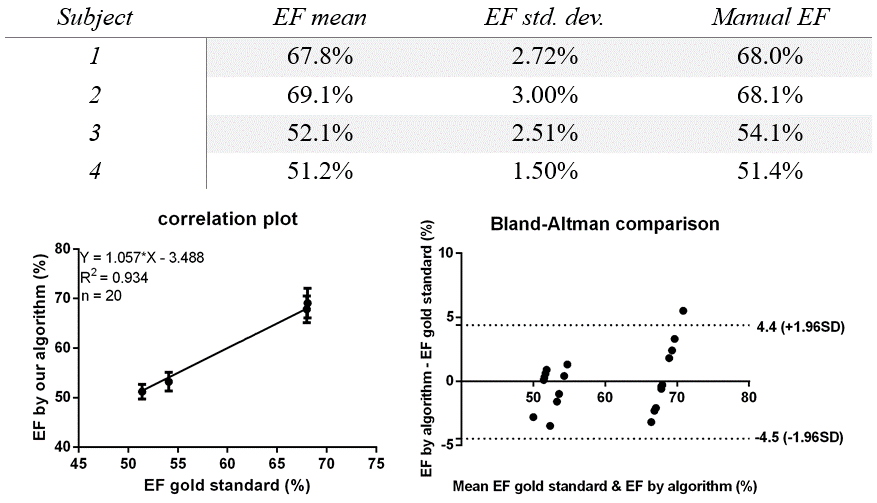
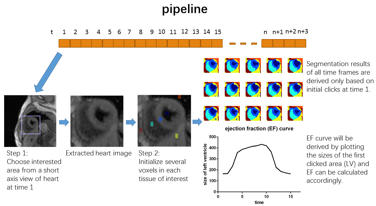
All image data were acquired on a 3T Siemens Verio scanner using T1/T2-weighted CMR multitasking6. The method was evaluated on four healthy volunteers. In each dataset, all T1/T2-weighted combinations were represented in the 25-dimensional tensor subspace which was already calculated during image reconstruction. The total image size before the segmentation was (160×160) voxels × 15 cardiac phases × 25 T1/T2-weighted features. Images were cropped and Θ was initialized by identifying several voxels in each tissue of interest. Image segmentation was then automatically performed, and EF was automatically calculated. The pipeline of the proposed method is shown in Fig.1.Results and Discussion
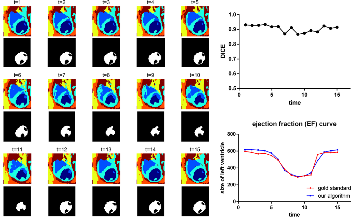
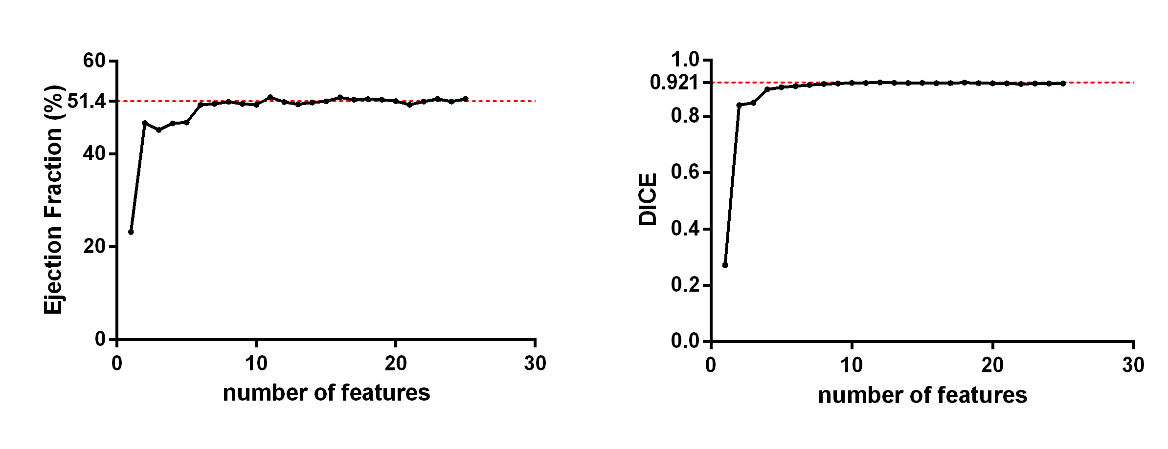
Segmentation was performed with five different initializations for each of the four datasets. Table 1 summarizes the overall results. The outcome shows a stable and accurate EF measurement as compared with manually segmented gold standards. The segmentation algorithm took approximately 1 minute to converge on a laptop computer running Windows 10 with an Intel Core i7 2.4GHz dual-core processor and 8GB RAM. A typical segmentation result is shown in Fig.2, which shows an accurate LV blood pool (for calculating EF) classification. All 25 contrast features were input into the algorithm in Fig.2; however, as few as 6 features may be enough to provide an accurate EF measurement as shown in Fig.3.Conclusion
In this study, a novel segmentation method for cardiac cine MR images has been developed, providing an efficient way to calculate EF. Our algorithm overcomes the noise and flow-dependent contrast distribution parameters commonly seen in cine MR images. Our algorithm is able to perform segmentation with small computational load in a predictable and stable way, potentially saving tedious manual work and providing low intra- and inter-observer variations. Future work includes extension to whole heart imaging, automatic initialization for fully automatic segmentation, and analysis of intra- and inter-observer variations.Acknowledgements
No acknowledgement found.References
[1] Steven C. Mitchell, et al. Multistage hybrid active appearance model matching: Segmentation of left and right ventricles in cardiac MR images. IEEE Transactions on Medical Imaging, pages 415–423, 2001.
[2] Honghai Zhang, et al. 4-D cardiac MR image analysis: Left and right ventricular morphology and function. IEEE Transactions on Medical Imaging, pages 350–364, 2010.
[3] J. Lötjönen, et al. Statistical shape model of atria, ventricles and epicardium from short- and long-axis MR images. MICCAI, pages 371–386, 2003.
[4] Zhi-Pei Liang. Spatiotemporal imaging with partially separable functions. IEEE-ISBI, pages 988–991, 2007.
[5] Anthony G. Christodoulou, et al. A general low-rank tensor framework for high-dimensional cardiac imaging: Application to time-resolved T1 mapping. Proceedings of the International Society for Magnetic Resonance in Medicine, page 867, 2016.
[6] Anthony G. Christodoulou, et al. Non-ECG, free-breathing joint myocardial T1-T2 mapping using CMR multitasking. Proceedings of the Society for Cardiovascular Magnetic Resonance, 2017.
[7] John Canny. A computational approach to edge detection. IEEE Transactions on Pattern Analysis and Machine Intelligence, pages 679–698, 1986.
[8] Yongyue Zhang, et al. Segmentation of brain MR images through a hidden Markov random field model and the expectation maximization algorithm. IEEE Transactions on Medical Imaging, pages 45–57, 2001.
[9] A. P. Dempster, et al. Maximum likelihood from incomplete data via the EM algorithm. Journal of the Royal Statistical Society, series B, pages 1–38, 1977.
[10] M. Proesmans, et al. Determination of optical flow and its discontinuities using non-linear diffusion. Proceedings of European Conference on Computer Vision II, pages 295–304, 1994.
[11] Thorvald Julius Sørensen. A method of establishing groups of equal amplitude in plant sociology based on similarity of species content and its application to analyses of the vegetation on Danish commons. Kongelige Danske videnskabernes selskab, pages 1–34, 1948.
Figures