4685
Automatic Segmentation of Human Brain MRI using Sliding Window and Random Forests1University of Edinburgh, Edinburgh, United Kingdom
Synopsis
Volumetric analysis of brain MRI acquired across the life course may be useful for investigating long-term effects of risk and resilience factors for brain development and healthy
INTRODUCTION
Quantitative volumes from brain MRI acquired at different stages of life offer the possibility of new insight into cerebral phenotypes of disease,and improved clinical decision-making and diagnosis. The literature presents a clear distinction between methods developed for different ages partly because the computational task is determined by properties of the acquired data and these are age-dependent1,2. Therefore, automated segmentation tools for modelling structure over years are lacking, and this hampers research that would benefit from robust assessment of the newborn to the adult trajectory. Here, we developed an automatic segmentation method for human brain MRI, where a sliding window approach and a multi-class random forest classifier were applied to high-dimensional feature vectors for accurate segmentation.METHODS
Data: The study included brain imaging data from 179 subjects, spanning the ages of 0–71 years, from three datasets. Dataset I.3 MR images and corresponding segmentation of 6 tissues/structures from 66 infants: 56 preterms (mean post-menstrual age [PMA] at birth 29.23 weeks, range 23.28–34.84 weeks) were acquired at term equivalent age ( mean PMA 39.84 weeks, range 38.00–42.71 weeks), and 10 healthy infants born at full term (> 37 weeks’ PMA). None of the infants had focal parenchymal cystic lesions. Ethical approval was granted by the National Research Ethics Service (South East Scotland Research Ethics Committee) and NHS Research and Development, and informed written parental consent was obtained. A Siemens Magnetom Verio 3T MRI clinical scanner (Siemens Healthcare GmbH, Erlangen, Germany) and 12-channel phased-array head coil were used to acquire T2-weighted (T2w) SPACE STIR: TR=3800ms, TE=194ms, flip-angle=120°, acquisition-plane=sagittal, voxel-size=0.9×0.9×0.9mm3, FOV=220mm, acquired-matrix=256×218. Dataset II.4,5 T1-weighetd (T1w) MRI and corresponding segmentation of 32 structures from 103 subjects (mean age 11.24 years, range 4.20-16.90 years). The images were acquired using a 1.5T Signa scanner (GE Medical Systems, Milwaukee, USA). Acquisition parameters: a 3-D inversion recovery-prepared spoiled gradient recalled echo coronal series, number-of-slices=124, prep=300ms, TE=1min, flip-angle=25°, FOV=240mm2, slice-thickness=1.5mm, acquisition-matrix=256×192, number-of-excitations=2. Dataset III.6 T1w MR images and corresponding segmentation of 32 structures from 18 healthy subjects including both adults and children; for the current study only adult data was used (N=10, mean age 38, range 35-71 years). Acquisition parameters: scanner/scan parameters unspecified, acquisition-plane=sagittal, number-of-slices=128, FOV=256×256mm, voxel-size=0.8-1.0×0.8-1.0×1.5mm3. Preprocessing: Brainmasks were provided with each dataset; except dataset I which was brain extracted using ALFA7. All images from all datasets were bias corrected using N48. Training data: To reduce the computational costs associated with learning, we used a sparsity-based technique to select a number of representative atlas images that capture population variability by determining a subset of n-dimensional samples that are ‘uniformly’ distributed in the low-dimensional data space7. Features: In addition to voxel intensities, we incorporated gradient-based features such as the norms of the first order derivatives and the norms of the second order derivatives. Sliding-window based classification: A sliding window was used to move over all possible positions in the test image, and for each window, the voxels inside the window are classified into different tissues or structures. The training samples come from the voxels of the aligned atlas images located at the same location as the voxels belonging to the test window. A local random forest classifier9 was then used to assign each voxel in the test image to a segmentation class. The feature extraction and classification framework is illustrated in Fig. 1. Evaluation: A leave-one-out cross-validation procedure was performed for every dataset. The comparison between automatic and reference segmentations was performed using Dice coefficient10.
RESULTS
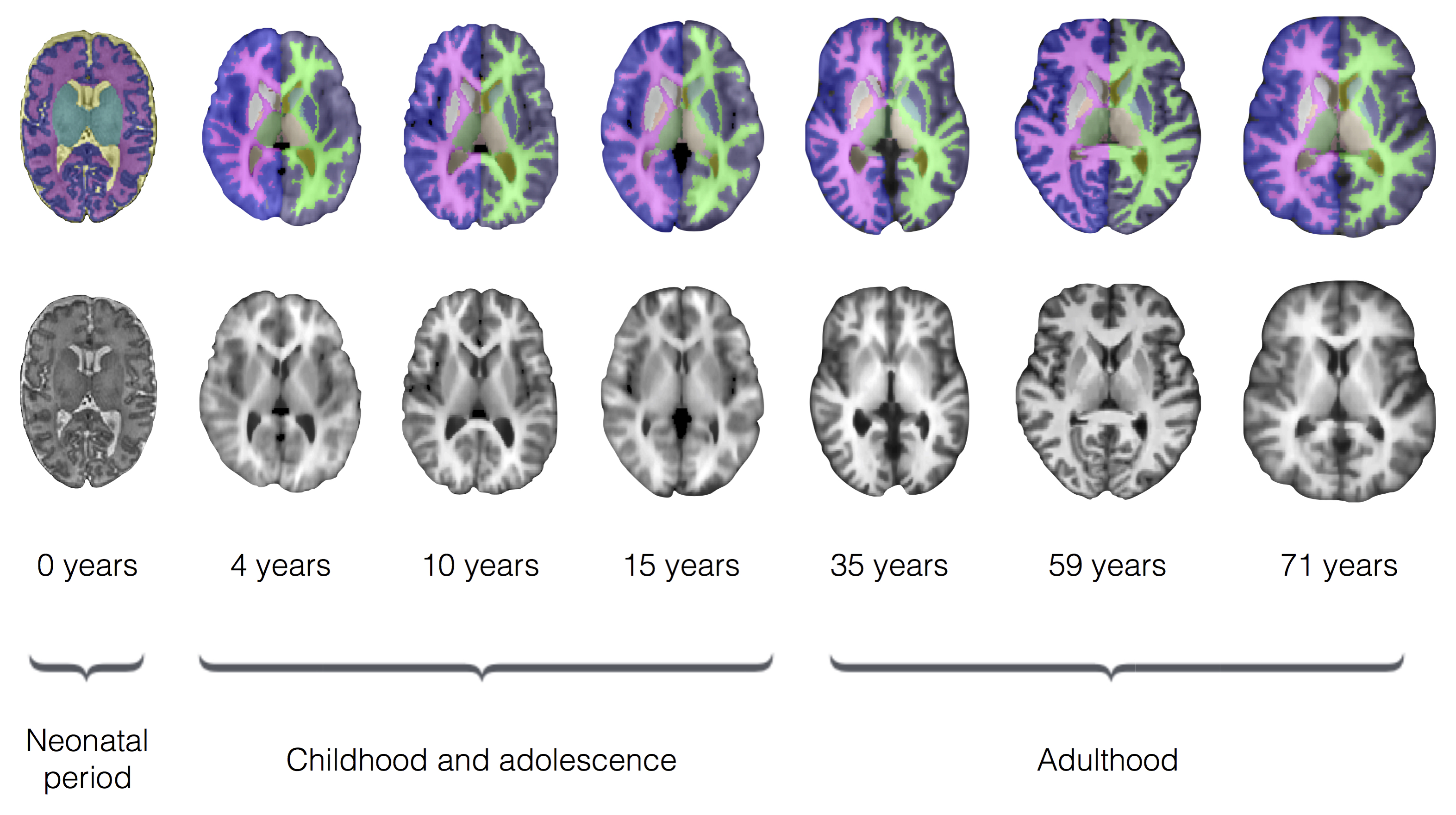
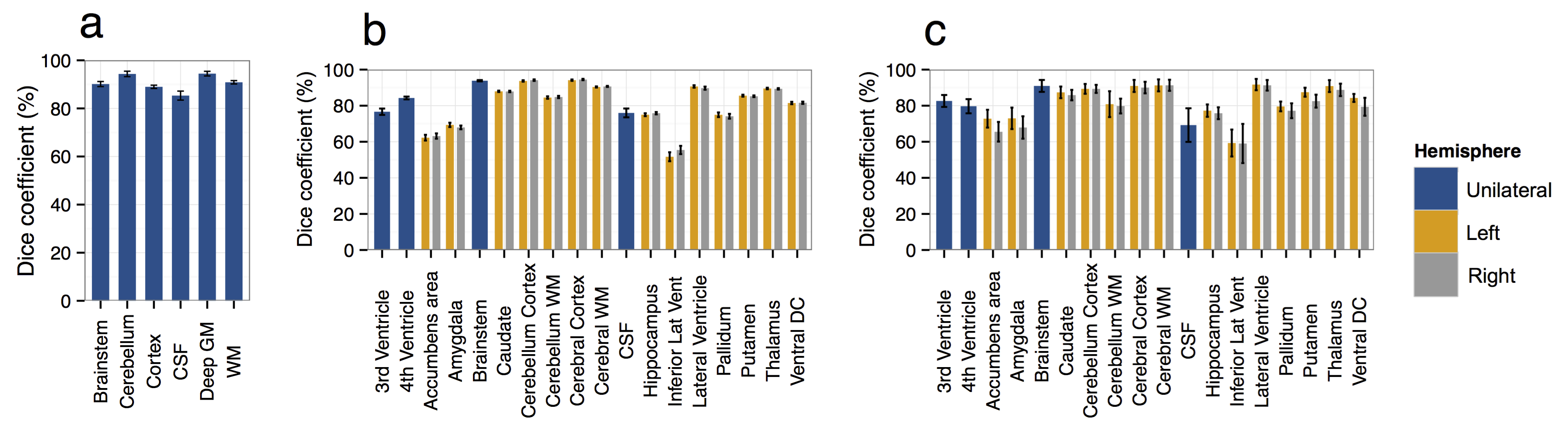
Figure 2 shows examples of brain segmentation results across the life course. Quantitative analyses (Fig. 3) indicated high accuracy for all tissues/structures with a mean Dice coefficient of 91% (dataset I), 86% (dataset II) and 83% (dataset III). We evaluated the influence of number of trees (nt) on segmentation accuracy. As the nt becomes large, segmentation accuracy increases, but training time increases and a threshold value is reached after which further improvement is not achieved (here nt=10). Regarding window size (w), the smaller w, the longer the classification time. Hence, w needs to be chosen carefully as it provides a balance between accuracy and speed (here w=5x5×5).
DISCUSSION AND CONCLUSION
We present a new method for MRI brain segmentation. The method was evaluated on three different datasets (span the ages 0–71 years) that provide different challenges to the brain segmentation task, and accurate results were obtained at all stages of development. As the method can learn from partially labelled datasets, it can be used to segment large-scale datasets efficiently. The method could also be applied to different populations and imaging modalities across the life course.Acknowledgements
We are grateful to the families who consented to take part in the study and to the nursing and radiography staff at the Clinical Research Imaging Centre, University of Edinburgh (http://www.cric.ed.ac.uk) who participated in scanning the infants. The study was supported by Theirworld, NHS Research Scotland, and NHS Lothian Research and Development. This work was undertaken in the MRC Centre for Reproductive Health which is funded by the MRC Centre grant MR/N022556/1.References
1. Cabezas, M., Oliver, A., Llado, X., Freixenet, J., and Cuadra, M. B., A review of atlas-based segmentation for magnetic resonance brain images. Comput Methods Programs Biomed, 2011. 104, e158-77.
2. Despotovic, I., Goossens, B., and Philips, W., MRI Segmentation of the Human Brain: Challenges, Methods, and Applications. Comput Math Methods Med, 2015. 450341.
3. Job, D. E. et al., A brain imaging repository of normal structural MRI across the life course: Brain Images of Normal Subjects (BRAINS). Neuroimage, 2016.
4. Kennedy, D. N. et al., CANDIShare: a resource for pediatric neuroimaging data. Neuroinformatics, 2012. 10, 319-22.
5. Frazier, J. A. et al., Diagnostic and sex effects on limbic volumes in early-onset bipolar disorder and schizophrenia. Schizophr Bull, 2008. 34, 37-46.
6. Rohlfing, T., Image Similarity and Tissue Overlaps as Surrogates for Image Registration Accuracy: Widely Used but Unreliable. IEEE Trans Med Imaging, 2012. 31(2): 153–163.
7. Serag, A. et al., Accurate Learning with Few Atlases (ALFA): an algorithm for MRI neonatal brain extraction and comparison with 11 publicly available methods. Sci Rep, 2016.
8. Tustison, N. J. et al., N4ITK: Improved N3 Bias Correction. IEEE Trans Med Imaging, 2010. 29, 1310-1320.
9. Breiman, L., Random Forests. Machine Learning, 2001. 45, 5-32.
10. Dice L. R., Measures of the Amount of Ecologic Association Between Species. Ecology, 1945. 26, 297–302.
Figures